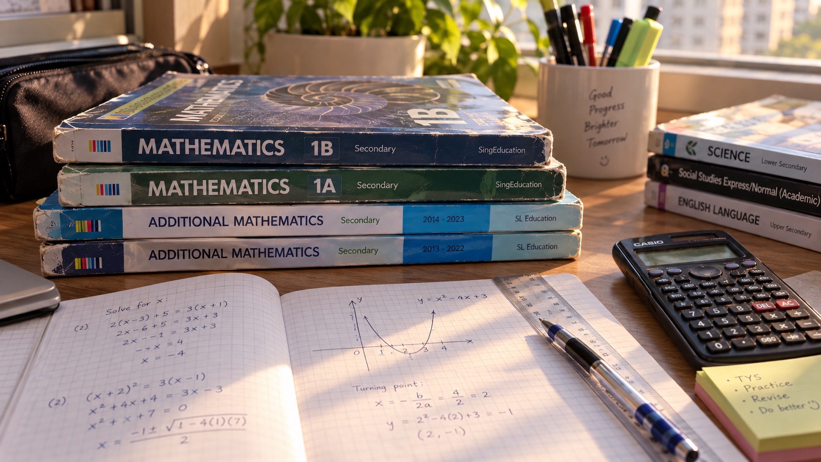
For a Punggol student admitted to secondary school through Posting Group 2 (PG2), G2 Mathematics statistics and probability can be learnt through practical questions: how to describe a group of values fairly, which average best represents the data, how spread changes the interpretation and what a chance calculation actually tells us. PG2 is an admission group, while G2 Mathematics describes an individual subject level under Full Subject-Based Banding. The student should follow the school’s actual subject offer and current topic sequence rather than assume every PG2 pupil takes an identical paper.

The 2027 Singapore-Cambridge Secondary Education Certificate G2 Mathematics K210 syllabus includes data handling, mean, median, mode, measures of spread, statistical diagrams and single and combined probability events. Those specifications apply to the 2027 graduating examination cohort, not a student first entering Secondary 1 that year. Families at Edgefield, Greendale, Punggol Secondary and Yusof Ishak Secondary can build the foundations using clearly hypothetical tables, counters, simple chance situations and critical questions about sampling, without inventing current statistics about Punggol residents or using real classmates as an unauthorised research sample. The important habit is to calculate correctly, explain the assumption and avoid overstating the conclusion.

• Posting group: PG2 is not a promise that every subject is taken at G2.
• Data: define what has been counted or measured before computing an average.
• Mean: add the values and divide by their number, or use frequencies appropriately.
• Median: order the data and find the middle value or midpoint of the two middle values.
• Mode: find the most frequent value, remembering ties and data sets without a mode.
• Spread: check range and later syllabus measures to understand variation.
• Probability: use all possible equally likely outcomes only when that assumption is justified.
• Combined events: distinguish mutually exclusive events from independent events.
• Next step: solve one small invented dataset and explain which average and chance model fits it.

Definition lock: statistical skill is different from the original posting route

Posting Group 2 guides admission to Secondary 1. G2 Mathematics is the level of the particular subject a student actually takes, and eligible pupils can offer different subjects at different levels under Full SBB. Statistics is a strand within Mathematics, not a separate type of posting group. A teenager’s aptitude with data may differ from their confidence with algebra or geometry, which is why a precise diagnosis matters more than a label.

The first family task is to confirm the actual textbook and class sequence. A Secondary 1 pupil may be learning basic averages while a graduating K210 candidate is expected to interpret standard deviation or combined probability. Presenting every advanced topic at once can confuse a learner who has not yet understood what the dataset represents. This article works from simple meanings towards more sophisticated ideas while preserving the distinction between foundational learning and later examination requirements.

What statistics is for

Statistics helps us describe variation and patterns in information. Instead of listing forty observations one by one, we may use a suitable table, graph or summary measure to make the data easier to understand. But summarising always involves choices. An average may conceal important differences, and a well-drawn chart may omit context. Students should ask how the data were collected and what question the summary is meant to answer.

A child might wish to describe the duration of fictional study sessions or the number of books in imagined groups. A short table can become useful practice without requiring personal information from real classmates. The correct interpretation begins by defining the group being studied, the units and the conditions. Mathematics then supports a reasoned statement. Statistics is not a machine that automatically turns any collection of numbers into a fact about the world.

The data source matters as much as the arithmetic

Before finding a mean or drawing a chart, ask whether the values are actual observations, official published figures, estimates or numbers invented for a teaching problem. Each category has a different evidential status. A mean calculated correctly from imaginary journey times is a valid answer to a hypothetical question, but it is not evidence of real LRT journey performance. A sample collected at one time may not represent every season or neighbourhood.

Teach the learner to label the source. If the task says ‘the following fictional observations’, keep that description in the interpretation. If the school supplies a genuine dataset, record its date and geographic scope. If information is missing, do not invent it to make a stronger conclusion. A careful mathematician values data provenance because an exact calculation can still produce a misleading claim when the underlying evidence is inappropriate.

Collecting, classifying and tabulating data

Data may be numerical measurements such as time and length, or categories such as a choice among three options. The type determines which summaries make sense. Calculating an arithmetic mean for arbitrary category names is not meaningful; counting their frequencies may be. Students should read the question and decide what each observation means before producing a table. Where labels or units are unclear, an answer may need to acknowledge that uncertainty.

Imagine an invented worksheet recording 2, 4, 4, 6 and 9 practice questions completed in five sessions. These are counts, so the sum, median and mode can be calculated. If the same worksheet instead lists five favourite genres, the meaningful summary may be frequency by genre. A learner who identifies data type first is less likely to apply a formula simply because a familiar keyword appears.

Mean: total divided by number of values

Take the fictional dataset 2, 4, 4, 6 and 9. The sum is 25 across five values, so the arithmetic mean is 5. It is important to write what five represents: the average count in this invented set, not five students or a real school statistic unless the question says so. The mean uses every value, which can make it sensitive to unusually high or low observations.

Ask the child to reconstruct the calculation from the definition rather than memorise a calculator sequence. If there were four observations instead of five, the divisor would change. If a number were recorded twice, it would influence the mean twice. Understanding the total and count prevents mistakes when the dataset is presented in a frequency table or a word problem rather than a simple list.

Median: order the observations first

For the ordered fictional values 2, 4, 4, 6 and 9, the median is the third value, 4. The median describes the middle of the ordered observations and is not calculated by adding the first and last numbers. If the dataset instead contains 2, 4, 6 and 10, the two middle values are 4 and 6, giving a median of 5. The method depends on the number of observations.

Students often forget to sort a jumbled list before selecting the middle item. Ask why the position rather than the size of the largest value determines the median. If one extreme observation becomes much larger, the median may stay the same even as the mean rises. This makes the median helpful for certain uneven datasets, but it does not mean it is always the best summary for every question.

Mode: the most frequent value

In the fictional set 2, 4, 4, 6 and 9, the mode is 4 because it appears twice while the other values appear once. A dataset can have more than one mode when values share the highest frequency. If every value occurs once, there is no unique most frequent value, often described as no mode in simple school examples. The mode is not automatically the largest number and is not found by dividing anything.

For categorical information, the most frequent category may be particularly useful, although the question should still be framed appropriately. A student can show frequencies in a clear table and identify which category appears most often. This does not establish why it is popular or whether it represents a larger population. The mode answers a frequency question; causal explanations require more evidence.

Choosing mean, median or mode

Suppose one fictional household budget dataset contains ordinary spending amounts plus one unusually high one-off purchase. The mean will increase because it includes the large observation, while the median may better represent the central position of routine spending. The mode may reveal a repeated amount but not describe typical financial pressure. No single average is universally superior. The aim is to choose the measure that answers the stated question.

Ask the child to justify the choice. If the problem concerns the total cost across several days, mean may be relevant alongside the total. If it concerns a typical value in a skewed dataset, median may be informative. If it concerns the most common category, mode may fit. Statistical understanding involves interpretation rather than simply computing all three measures and hoping one is marked correct.

Outliers can change a summary dramatically

Imagine two fictional sets of four durations. Set A is 10, 11, 12 and 13 minutes; Set B is 10, 11, 12 and 47 minutes. Their means are 11.5 and 20 minutes respectively. Yet the medians are 11.5 and 11.5 minutes. The long final observation changes the mean substantially without changing the middle pair. That is a useful example of why reading only one summary can mislead.

The correct response is not to delete the 47-minute observation merely because it changes the average. It may be genuine, a recording error or an unusual condition. The learner should identify what is known and what would need checking. Good data analysis uses unusual values as questions to investigate, not inconveniences to conceal. The calculations here use invented numbers and describe no real Punggol journey.

Range gives a first measure of spread

The range of a numerical dataset is the largest value minus the smallest. For 2, 4, 4, 6 and 9, the range is 9 − 2 = 7. The range reveals the overall span, but it does not say where most observations lie or how frequently extreme values occur. Two datasets with the same range can have very different patterns. A student should use the range as one part of a description, not as a complete account of variation.

Ask what changes when a single unusually high observation appears. The range may increase dramatically while most values remain clustered. This connects the idea of spread with the earlier discussion of outliers. A learner who can distinguish central tendency from variation is already thinking statistically rather than treating every dataset as one number.

Quartiles and the interquartile range come later

The 2027 graduating K210 syllabus includes quartiles and percentiles, as well as range and interquartile range. These ideas describe positions and spread within ordered data, with the interquartile range representing the difference between upper and lower quartiles under the specified convention. Students should follow their actual school method for handling small datasets and quartile positions, as teaching and assessment conventions matter in particular exercises.

The important conceptual point is that the middle portion of data can be analysed separately from extreme values. A box-and-whisker plot makes such information visible. But a Secondary 1 pupil who is still unsure how to order numbers and find the median should stabilise those skills first. Advanced summaries make sense only when the foundational data concepts are understood.

Standard deviation is not just a harder word for range

The graduating G2 Mathematics K210 syllabus also includes standard deviation as a measure of spread. Unlike range, standard deviation uses how values vary around the mean, according to the syllabus formula. A larger standard deviation generally indicates greater dispersion under comparable conditions. However, it should not be confused with average value or the total amount of data. A low standard deviation does not prove a dataset is accurate or representative.

Parents can introduce the idea using two simple fictional sets with the same mean but different spreads. One set has values close together; another is more dispersed. The exact computation belongs at the appropriate point in the school sequence. The conceptual foundation is understanding why the mean alone may be insufficient and how variation affects confidence in interpreting numerical results.

Grouped data requires a frequency-weighted mean

When values are displayed in a frequency table, adding each distinct value once and dividing by the number of rows is usually incorrect. If a value of 2 occurs three times and a value of 5 occurs once, the four observations total 2 + 2 + 2 + 5 = 11, giving a mean of 2.75. The frequency-weighted calculation is (2 × 3 + 5 × 1) ÷ 4. This reflects all observations.

Ask the child to expand a small frequency table into its original data list and compare the two methods. That demonstration makes the formula meaningful. The frequencies tell us how many observations each value represents, not merely how many labels appear in the table. Later, grouped intervals may require additional assumptions or midpoint approximations under the syllabus’s methods. Avoid treating every grouped table as if it contained exact raw values.

A chart is a representation, not the data itself

Bar graphs, line graphs, pie charts and other displays make certain features visible. But they can also conceal individual values or emphasise a difference depending on scale and design. Students should choose a display suited to the variable and question. A bar chart can compare categories; a line graph may suit repeated measurements over time; a pie chart concerns parts of a whole. The correct choice depends on what the observations mean.

This article’s focus is selecting and interpreting statistical summaries rather than repeating the separate PG2 guide to everyday graphs. Ask which comparison the chart helps answer and what important information remains hidden. A graph may communicate the same data more clearly for one purpose and less clearly for another. The student should understand why the representation was chosen.

A pie chart must represent a complete whole

Pie charts divide a circle into sectors corresponding to shares of a complete total. If a fictional class preference table has twenty responses, five in one category represent one-quarter of the responses, or 25%. That would correspond to a sector of 90 degrees. The shares of mutually exclusive, exhaustive categories should account for the whole when the categories are defined properly.

A common error is to interpret the largest sector as proving that most of the whole population holds that view. The chart might show only twenty hypothetical respondents from one group. A pie chart can accurately describe the sample and still be insufficient for generalising. Ask the learner to state the denominator and whether the categories overlap. Geometry and statistics meet in the sector angles, but statistical validity requires more than correct drawing.

Sampling determines how much confidence is appropriate

A small or selectively chosen group may not represent the larger population. Suppose a fictional student asks only friends who play one sport what their favourite activity is. The resulting sample is likely to overrepresent that sport compared with the entire school. The student can report accurately what those friends said, but should not claim it describes every teenager in Punggol. The flaw concerns the sampling method, not the arithmetic.

Teach the child to ask who was included, how participants were chosen and who was excluded. If a real school project requires a survey, follow the teacher’s privacy and consent procedures. Do not collect identifiable classmates’ opinions or publish raw responses without authorisation. Fictional datasets or trusted public statistics can teach the principles safely. Responsible sampling is part of Mathematics literacy, not just a research ethics issue.

Percentages need the correct denominator

Imagine a fictional table where twelve of thirty students choose an option. The observed proportion is 12/30 = 0.4, or 40%. The denominator is the thirty responses considered, not the entire school unless the question states that all school students participated. If some respondents could choose multiple options, the shares might sum to more than 100%, which can be valid in that different survey design.

Ask the learner to describe the population and sampling conditions before making a percentage claim. It is possible to calculate 40% correctly and then write an invalid statement such as ‘40% of all Punggol teenagers prefer it’. The original evidence supports only the fictional sample. Quantitative accuracy and honesty about scope must travel together.

Probability is a measure of chance

Probability assigns values from zero to one to describe the likelihood of events under a model. A probability of zero means an event is impossible in that model; one means certain; one-half means a 50% chance. Such statements depend on how the situation is defined. A probability of one-half does not guarantee that an event happens exactly once in every two trials.

Ask the child to describe the possible outcomes before writing a fraction. An ideal fair coin offers two equally likely outcomes, but the model includes assumptions about the coin and toss. Not every real-world situation can be reduced to a fair two-outcome model. The critical skill is identifying the sample space and the conditions that make a probability calculation valid.

Equally likely outcomes must be justified

A student may write probability as favourable outcomes divided by all outcomes. That simple counting formula works when the elementary outcomes being counted are equally likely. If a spinner has sectors of unequal area, counting colours without considering the sizes may be wrong. If a bag has different numbers of coloured counters, counting colours rather than individual counters also changes the model.

For example, a fictional bag contains three red counters and one blue counter, with each counter equally likely to be drawn. The probability of red is 3/4, not 1/2 merely because there are two colours. Ask the child which objects are equally likely and how many belong to the event. A small physical or drawn model can prevent an incorrect denominator. All objects in this example are imagined teaching materials.

The complement helps check a probability

If event A has probability 0.3, the probability that A does not occur is 0.7, assuming those are complementary alternatives within the same complete event model. The two probabilities sum to one. This relationship can help solve questions where counting the opposite event is easier, but the student must identify the complement correctly. ‘Not choosing red’ may include several other colours, not just blue, if more categories exist.

Ask the child to list all allowed outcomes and mark the event and its complement. When the groups cover the whole space without overlap, their probabilities add to one. This is a useful verification step. A probability answer outside zero to one or a purported complement that omits outcomes signals an error in the model.

Mutually exclusive events cannot happen together

Two events are mutually exclusive if they cannot both occur in the same trial. On one roll of a standard fair six-sided die, the events ‘roll a 2’ and ‘roll a 5’ cannot occur together. Their probabilities add when asking for a 2 or 5: 1/6 + 1/6 = 1/3. This addition is justified because the events do not overlap.

By contrast, ‘roll an even number’ and ‘roll a number greater than 3’ overlap on 4 and 6. Simply adding their probabilities would count those outcomes twice. Ask the learner to list the sample space and draw overlapping sets when needed. The key is understanding overlap before choosing a formula. Vocabulary such as mutually exclusive should clarify the model rather than serve as a memory trick.

Independent events describe a different relationship

Two events are independent when knowing one has occurred does not change the probability of the other under the model. For two ideal independent fair coin tosses, the probability of heads on both is 1/2 × 1/2 = 1/4. A student should list the four equally likely ordered outcomes: HH, HT, TH and TT. The single favourable outcome gives the same result.

Independence is not the same as mutual exclusivity. The two coin-toss results can both be heads; they are not competing alternatives. In contrast, drawing two counters from a bag without replacement often changes the contents and therefore changes probabilities for the second draw. Teach the child to read whether replacement occurs and whether the question genuinely establishes independence.

Tree diagrams reveal sequences

A tree diagram can organise the possible results of two stages and show conditional probabilities along each branch. For an ideal coin tossed twice, the first stage branches into heads and tails, and each of those branches again into heads and tails. The probability of a particular ordered path is found by multiplying branch probabilities when the model warrants it. The complete set of final outcomes should account for probability one.

Ask the teenager to explain what each branch represents. The diagram is not a decorative substitute for thinking; it is a way to avoid omitting outcomes and to preserve sequence. For without-replacement situations, the branch probabilities may change after the first event. A student who copies 1/2 onto every branch without considering the process has misunderstood the model.

An example with a counter drawn without replacement

Imagine a fictional bag with two red counters and one blue counter. Two counters are drawn sequentially without replacement. The probability of drawing red first is 2/3. Given that the first draw was red, the probability of red second is 1/2. The probability of red on both draws is therefore 2/3 × 1/2 = 1/3. The second factor differs because the bag’s contents have changed.

This small example shows why the phrase ‘without replacement’ matters. A learner who multiplies 2/3 by 2/3 would ignore the first draw’s effect. Ask the child to recount the remaining counters after each branch. When the physical logic is clear, the multiplication becomes understandable. No real classroom survey, gambling or purchase is involved; this is an elementary counting model.

Fair games should be judged using the complete rules

A game may advertise a large reward while offering a small chance of winning. Probability can help explain the difference between a possible outcome and an expected result, but students should not be encouraged to gamble or interpret a hypothetical exercise as a recommended betting activity. In school, safe examples use imaginary counters, fair dice or classroom simulations. The focus is understanding outcomes and fairness of the rules.

Ask whether the model provides equal opportunities and whether the outcomes have been counted accurately. A fair coin is a mathematical ideal; real objects can have imperfections. Repeated trials may approximate theoretical proportions without guaranteeing that small samples match exactly. A strong student can describe both the theoretical chance and the uncertainty of an observed sequence.

A run of one result does not prove the next result is due

Suppose an ideal fair coin comes up heads four times in a row. Under the model of independent tosses, the probability of heads on the next toss remains one-half. The previous sequence does not make tails ‘due’. This is a useful opportunity to teach independence and the difference between long-run frequencies and predictions about one trial.

The learner can list outcomes or use a simple simulation to explore the idea. But a small sample can look uneven by chance. An accurate explanation should avoid claiming that all sequences must alternate or that a long run changes the coin’s underlying fairness. Understanding chance includes accepting that random processes do not always look balanced in short intervals.

Experimental frequency and theoretical probability are distinct

Theoretical probability is calculated from a specified model, such as equal outcomes on a fair die. Experimental relative frequency is obtained from observed trials. If a fictional experiment produces seven heads in ten tosses, the observed frequency is 70%, even though the ideal theoretical probability of heads is 50%. The difference does not automatically prove that the model is wrong.

Ask what happens when the number of trials increases and why the observed proportion might fluctuate. Do not alter the recorded results to match the expected fraction. Mathematics can describe uncertainty honestly. It is possible for a finite sequence to deviate from the theoretical probability, and responsible interpretation recognises that distinction instead of treating every unexpected run as evidence of a conspiracy.

Statistics and probability can work together

A school task may use a dataset to estimate how often an event occurred and compare it with a theoretical chance model. The learner should identify whether the situation is descriptive or predictive and whether the necessary assumptions hold. A table of observed outcomes does not automatically define equal probabilities for future outcomes. Conversely, a theoretical model does not guarantee that every observed sample will perfectly match it.

Ask the student to state what is known, what is assumed and what is being inferred. A clear comparison may show how many times a result occurred in a fictional experiment and how that relates to the probability under an ideal model. The quality of the reasoning matters more than whether the numbers happen to agree closely. Good mathematical literacy combines calculation with the limits of evidence.

Punggol contexts should be identified as fictional or verified

A family might use a hypothetical table of LRT waiting times, library borrowing choices or community activity attendance to make statistics feel familiar. But such invented numbers must not be presented as real operational data about Punggol. A student may calculate the mean of a fictional route-time dataset, yet that does not establish the average commute of residents or whether a transport service is reliable.

For real local factual claims, use appropriate published datasets and note the period, definitions and geographic scope. If a child collects data for a genuine school assignment, follow consent and safety instructions. There is no need to record strangers or gather sensitive personal information to learn an average or probability. Imagined numbers can support excellent mathematical instruction as long as their evidential status remains clear.

A fictional student chooses the wrong average

Imagine a fictional teenager, Hana, analysing four monthly spending observations with one unusually large event cost. She calculates the mean correctly and tells her parent it represents an ordinary month. Her parent asks whether the one-off cost has changed the summary. Hana orders the observations, calculates the median and notices that the two measures communicate different aspects of the data.

She revises her explanation to state what the mean includes and why the median may be informative for a typical month. The example is invented, not a real family financial profile. It demonstrates that the correct arithmetic does not automatically provide the best interpretation. A learner must choose the measure in relation to the question and describe any unusual values honestly.

A fictional student forgets that draws change the bag

Imagine another learner, Amir, working with a hypothetical bag of coloured counters. He calculates the chance of drawing red twice without replacement by multiplying the initial red proportion by itself. His teacher asks him to count what remains after the first red is removed. Amir sees that the second probability must use the updated total and colour count.

He then solves a related example in which the counter is replaced between draws and explains why the probabilities differ. The improvement is conceptual: he can now identify a condition that changes the mathematical model. This invented scenario contains no live game or gambling activity. It shows how a short discussion about assumptions can be more effective than repeating a formula without meaning.

A two-week practice route from averages to chance

During the first days, practise identifying the data type and calculating mean, median, mode and range from small fictional datasets. Then compare two sets with the same mean but different spread. Next, use clear tables and charts to discuss misleading summaries and sampling limitations. During the second week, list outcomes for simple chance situations and practise complementary, mutually exclusive and independent events at the difficulty appropriate to the school syllabus.

End with an unfamiliar word problem where the student must decide whether the task asks for an average, a frequency or a probability. The sequence is optional and should not be forced ahead of the current school curriculum. If basic fractions are insecure, repair that prerequisite first. Meaningful progress occurs when the teenager chooses a valid model and explains it without hints.

How to correct a statistics or probability mistake

Some wrong answers are arithmetic errors. Others arise from using the wrong denominator, forgetting to order data, treating categories as numbers or assuming equally likely outcomes without justification. A tutor should identify the first incorrect decision and teach that specific concept. More questions of the same kind may help only after the learner understands the correction. A student who copies a complete worked solution may reproduce the answer without learning why it is valid.

Use a correction record with the original error, its cause and a contrasting new task. For a median mistake, change the number of observations. For a probability mistake, change whether an item is replaced. The learner should explain how the model changes. That independence is a stronger sign of learning than the total number of worksheets completed.

The G2 K210 syllabus is a long-term map, not a Secondary 1 checklist

SEAB’s 2027 graduating K210 Mathematics syllabus includes statistical representations, measures of spread and both simple and combined probability. Not all of those ideas are appropriate for a new Secondary 1 pupil in the same term. The school determines the actual lower-secondary sequence and level. Families should use the national document to understand the pathway while respecting the learner’s present prerequisites.

A child who understands why mean and median differ is better prepared for quartiles and standard deviation later. A teenager who can list fair-die outcomes correctly has a more stable foundation for tree diagrams. Rushing ahead can obscure these relationships. Good teaching builds durable concepts and tests them in unfamiliar situations before adding complexity.

Sources, related guides and your next step

Use SEAB’s 2027 G2 Mathematics K210 syllabus for the Statistics and Probability strand and the official 2027 G2 syllabus index to confirm the graduating cohort. For the curriculum-level distinction, refer to MOE Full Subject-Based Banding. Each Punggol secondary school communicates its own present Mathematics teaching scope.

The earlier PG2 ratios, percentages and graphs guide covers different numerical applications, and the algebra guide covers equations. Your next step is to give the student one invented dataset, ask which average best answers a stated question, then create a simple counter-draw problem and require the learner to explain why the sample space and probabilities are valid.

Frequently asked questions about PG2 G2 statistics and probability

Does PG2 mean every student must take G2 Mathematics?

No. PG2 is the admission grouping; check individual subject-level offers under Full SBB.

What is the difference between mean, median and mode?

Mean averages the numerical total, median identifies the central ordered value or pair, and mode identifies the most frequent value.

Can a dataset have no mode?

Yes. In a simple dataset where every value occurs equally once, there is no unique most frequent value.

Why might median be more representative than mean?

An unusually high or low observation can change the mean substantially without similarly affecting the median.

What does range measure?

The difference between the largest and smallest numerical observations, not the complete distribution.

When is favourable outcomes divided by total outcomes valid?

When the elementary outcomes being counted are equally likely under the stated probability model.

Are mutually exclusive events the same as independent events?

No. Mutually exclusive events cannot coincide; independent events do not change one another’s probability under the model.

Does drawing without replacement affect the next probability?

It can. The composition and total change after an item is removed.

Does a run of coin toss heads make tails due next?

No. Under an ideal independent fair-coin model, the next toss remains equally likely to be heads or tails.

What is an appropriate Punggol practice dataset?

Use clearly invented numbers or properly sourced public data, never pass fiction off as measured local statistics.

Editorial note: Published 1 November 2026. All survey counts, prices, journey durations and student stories identified as fictional are teaching examples, not official Punggol data. K210 refers to the 2027 graduating SEC cohort; the student’s current school syllabus controls the lower-secondary topic sequence.