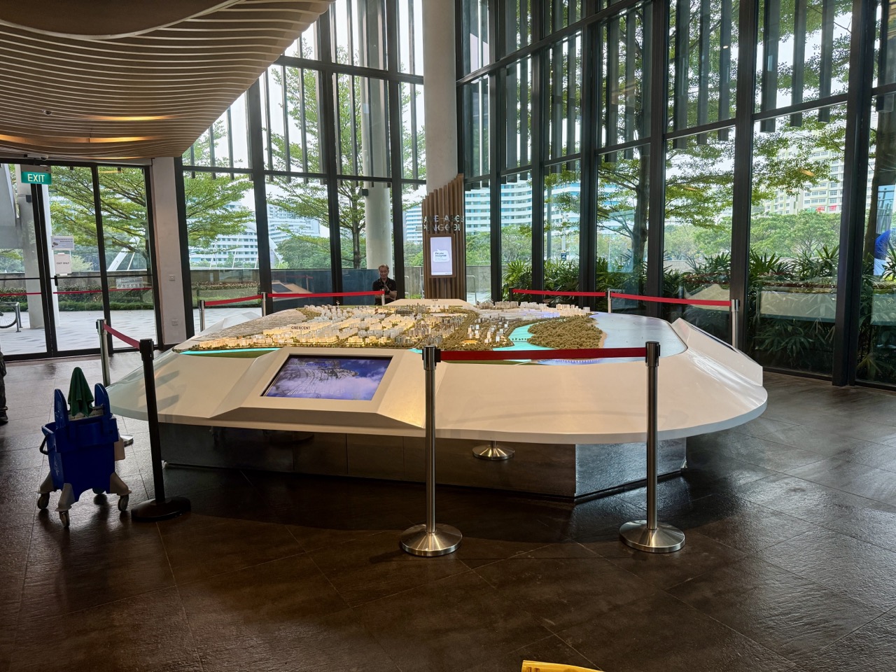
The top 10 things to do in Punggol for Data Science students are to interpret SingStat’s June 2026 planning-area dataset, read NEA PM2.5 data through data.gov.sg’s documented API, clean missing and duplicated values, join MRT/LRT station names accurately, distinguish opened from planned Heritage Trail geometry, test sampling bias using hypothetical visitor data, chart age distributions with correct denominators, separate JTC solar forecasts from measured outputs, apply PDPC anonymisation principles and build a fully documented mini-dashboard.

Best starter project: use a five-row fictional air-quality table and make one chart that preserves timestamps, units and missing readings. For genuine public information, use SingStat’s June 2026 geographic distribution and data.gov.sg’s documented NEA regional API. Do not treat a North-East regional value as a measurement at your Punggol block, and never let a student dashboard appear to be an official live health or travel service.

This October 2026 guide is different from a generic Statistics or Computer Science article. It teaches an end-to-end data pipeline—finding trustworthy sources, reading schemas, checking units, joining keys, cleaning records, understanding sampling, interpreting projections, protecting privacy and documenting reproducible results. Every worked number is fictional or a labelled calculation from an attributable source; current opening, service and environment claims must be rechecked before use.

Choose the correct data skill for the problem

• Data discovery: find the original SingStat or data.gov.sg file, not a copied screenshot.
• Schema reading: identify rows, dimensions, counts, units and total or subtotal entries.
• Cleaning: preserve true missing values and flag duplicates before analysis.
• Joining: use exact station codes or other stable identifiers, not ambiguous text fragments.
• Spatial data: distinguish a planned line on a map from a publicly open route.
• Sampling: ask who and what a dataset actually represents.
• Visualisation: choose readable axes, honest denominators and appropriate dates.
• Forecast evaluation: separate projected district performance from measured data.
• Privacy: minimise collection and assess re-identification risks.
• Reproducibility: write enough method detail for another learner to check the result.

The data science workflow begins with a defined question

A vague project such as ‘analyse all of Punggol’ is too wide for a meaningful first dataset. A narrower question might ask how an age-category total relates to a planning-area population, whether a time series contains missing hourly PM2.5 observations, or which station code actually corresponds to a public destination. A good question determines the correct source, level of detail and analysis. A fashionable model cannot repair the wrong question or a mismatched denominator.

Before using any value, preserve the source identity and date. For SingStat, the June 2026 release describes population at a particular reference point. For data.gov.sg real-time readings, a timestamp and region are fundamental. For JTC’s sustainability estimates, a target or projection must not become a current measured output just because it is displayed with a large number. Those fields are not decorative metadata: they are part of the truth of the claim.

The complete workflow should be visible to a reviewer. Identify the source and licence, read the data dictionary, inspect missing and duplicate fields, make documented transformations, test the resulting values, choose a suitable chart, explain uncertainty and record one correction. In this form, a simple spreadsheet can be more rigorous than an elaborate dashboard that hides invented assumptions.

Ten Punggol data science learning investigations

Read a 2026 SingStat Punggol planning-area table like a dataset

Where: Singapore Department of Statistics geographic-distribution data, released for June 2026.

Why this dataset or problem matters

SingStat provides CSV and Excel tables with Singapore residents by planning area or subzone, age group, sex and dwelling characteristics. Its Population Trends 2026 report identifies Punggol among areas with a high relative proportion of children under five. The central data-science task is reading a dataset’s unit of analysis and schema before producing a visualisation. ‘Punggol planning area’, a subzone, a constituency and an individual flat are different geographic units. A date or total resident population is equally essential to the correct interpretation.

Build the exercise step by step

Start from SingStat’s current Geographic Distribution page and locate the June 2026 downloadable table, preserving the original source name and retrieval date. Open a copy in a suitable safe spreadsheet environment, and identify which columns are dimension labels, which are values, and whether totals or subtotals appear as separate rows. On a private working copy, filter only the intended Punggol planning area and chosen age categories. Do not sum a total row together with its constituent age groups. Build a short data dictionary stating the meaning and unit of each field.

Original worked example and common error

Fictional illustration: an age table contains groups A=20, B=30 and a separate ‘Total’=50. A learner uses a pivot that sums all rows and reports 100 residents. The total has been counted twice. The corrected pipeline either selects the aggregate total or computes 20+30, not both. Actual Punggol demographic numbers must come from the SingStat file, not these made-up figures.

Improve and extend the analysis

Ask how age bands, resident definitions and geographic boundaries could change over time. A comparison with 2025 should preserve compatible fields and account for revisions. Build an automated check that age-band subtotals equal the official total when the dataset structure warrants it. If the relationship fails, investigate suppression, rounding and missing categories before assuming corruption. Explain why a program that imports a file is not yet a validated demographic analysis.

Evidence, access and privacy boundaries

Aggregated population statistics cannot identify the family structure, ethnicity, income or health of any individual observed in Punggol. Protect the source’s licence and attribution. Do not treat a planning-area statistic as a personal prediction.

Official source: Read a 2026 SingStat Punggol planning-area table like a dataset. Preserve its actual data version and context.

Make a clean PM2.5 time series from data.gov.sg’s API contract

Where: Data.gov.sg’s documented real-time NEA PM2.5 interface, viewed from home or library.

Why this dataset or problem matters

Data.gov.sg documents hourly NEA PM2.5 observations for Singapore’s major reporting regions, with a timestamp, regional metadata and concentrations in micrograms per cubic metre. Unlike a static park directory, this is a changing time series. Data Science students need to preserve timezone, units, update frequency and actual observed response values. The North-East regional label cannot be silently converted into an exact sensor reading at Punggol Waterway, a school or a home.

Build the exercise step by step

Read the official API specification before attempting any request. Document its endpoint, date filter, response structure, pagination where applicable and current authentication or rate-limit requirements. Beginners can work from a hypothetical CSV with the same field concepts. More advanced authorised users may call the official API within its documented terms, retain the response timestamp, select a single region and plot the values chronologically. Put units and time on axes, and show the last verified update prominently.

Original worked example and common error

Fictional data points of 15, 18 and 21µg/m³ at three distinct hours form a steadily rising line, but the simple average of 18µg/m³ says nothing about indoor exposure and cannot be identified as current data. A student who labels the chart ‘Punggol Block 123 live PSI’ has made multiple mistakes: invented local precision, substituted PSI for PM2.5 and implied real-time freshness. The corrected title states region, metric, unit, synthetic-data status and dates.

Improve and extend the analysis

Test a timezone offset, a missing hour and an API error. Describe whether the visualization should show a gap, a dated cached value or an explicit failure. A resilient dashboard never takes yesterday’s data and silently changes its label to ‘now’. Study why hourly samples can contain spikes and why smoothing over a longer window changes what the graph communicates.

Evidence, access and privacy boundaries

Follow API terms, authentication, source attribution and rate limits. Do not publish private keys or present classroom numbers as live NEA readings. Real haze decisions require current official advisories rather than experimental analysis.

Official source: Make a clean PM2.5 time series from data.gov.sg’s API contract. Preserve its actual data version and context.

Detect missing values and double-counted records before analysis

Where: A wholly fictional Punggol environmental dataset processed offline.

Why this dataset or problem matters

Cleaning data is not simply deleting inconvenient rows. A missing observation may be caused by a paused sensor, inaccessible record or broken data transfer, while a true zero means the quantity was observed as zero. Duplicate records can have identical or conflicting values, and a data file may include totals alongside the component records. An honest analyst must decide what each unusual field means and document every decision before calculating a trend.

Build the exercise step by step

Create a six-row fictional dataset with one missing measurement, one repeated timestamp and an invalid text entry in a numeric field. Mark the entire file ‘training data’. Write validation rules: an observation has a parseable timestamp, expected unit, allowed region and numeric concentration or explicit null state. Sort by time and flag duplicates for review instead of automatically retaining the latest row without reason. Track the number of rows before and after each step in a cleaning log.

Original worked example and common error

Illustrative accepted numeric values are 10, 12, 20 and 18, plus a missing entry. Their mean is 15 from four valid numbers; treating the missing entry as zero and dividing by five produces 12. The two means answer different questions. A junior analyst initially chooses 12 because their code fills blanks automatically; the correction asks whether ‘zero’ was ever measured. The result is an explicit null-preservation policy.

Improve and extend the analysis

Add a duplicate time with a conflicting numeric value. Discuss possible policies, such as marking the row for source review, and the metadata needed to decide which is authoritative. Construct unit tests for an empty file, invalid timestamp, mixed units and a total row inserted unexpectedly. Reproducible cleaning is a documented decision process, not a hidden series of button clicks.

Evidence, access and privacy boundaries

Do not invent environmental measurements to make a prettier published chart. Data quality work cannot diagnose source-system problems without actual evidence, and student scripts must not scrape or overload government APIs.

Official source: Detect missing values and double-counted records before analysis. Preserve its actual data version and context.

Join official Punggol MRT and LRT place names without mixing stations

Where: LTA current rail-network information and public route diagrams.

Why this dataset or problem matters

A join connects records that refer to the same entity. Punggol MRT NE17, Punggol Coast MRT NE18 and Punggol Point LRT PW3 sound similar but are not interchangeable keys. In data analysis, a text join on the word ‘Punggol’ can create false matches or duplicated rows. A transport geography project therefore needs a stable station identifier, correct network and valid temporal status for every link. Current service and future Cross Island Line plans must be separated.

Build the exercise step by step

Build a small table with station code, official full name, line or loop and operating status, drawing from current LTA pages. Make a second fictional table of visitor destinations keyed to a verified station or an explicit null if no direct station is documented. Join on the complete station code, not on the shared word in the name. Check row counts before and after to spot unwanted many-to-many matches. Avoid inventing distances or live travel times from a schematic drawing.

Original worked example and common error

Table A contains NE17 Punggol and NE18 Punggol Coast; Table B contains a destination called ‘Punggol Coast Mall’. An imprecise substring join assigns the mall to both stations, while a properly documented location relationship identifies its relevant Punggol Coast approach. This is an entity-resolution lesson; the workbook does not guarantee a current walking route or accessible exit.

Improve and extend the analysis

Add a future planned Riviera Cross Island Line field with a status of ‘not operational in this dataset’. Test whether a route algorithm mistakenly treats it as currently usable. Create a validation rule requiring an effective date for status changes, and ask why a route published in 2023 might not be accurate in 2026.

Evidence, access and privacy boundaries

Do not claim exact fares or lift status from a station-code table. Travel decisions require live LTA and operator information, and nothing in a public map authorises access to railway systems.

Official source: Join official Punggol MRT and LRT place names without mixing stations. Preserve its actual data version and context.

Compare mapped distance with real public access at the Heritage Trail

Where: JTC Punggol Heritage Trail’s first confirmed opened section near Punggol Coast.

Why this dataset or problem matters

JTC currently confirms the first 400 metres of the planned 1.3-kilometre Punggol Heritage Trail as open. The separate lengths provide a simple example of geographic data with different operational statuses. A line on a future planning map and a line representing a lawful presently opened path cannot be placed in the same ‘available route’ field without a qualifier. A data scientist should include planned versus operating status, date and uncertainty before using the geometry for a visitor itinerary.

Build the exercise step by step

Read the current JTC community page and the 2025 NParks opening notice. Create a conceptual geographic table with feature name, reported length, current operational status, source and last-reviewed date. Sketch the current opened section in one line style and the planned full alignment in another. For a simulated route query, return only verified open links and warn when the requested destination needs a later phase. If actual path data are unavailable, do not draw precise coordinates from a conceptual illustration.

Original worked example and common error

A student enters 1.3km into a route-planning spreadsheet and reports a guaranteed twenty-minute stroll from one end of the future trail to the other. JTC’s operational information confirms only 400m as opened in the cited stage. The corrected model does not promise through-access; it describes the currently confirmed section and marks other segments as needing future verification.

Improve and extend the analysis

Explain the difference between Euclidean distance, network path length and published trail length. Ask why a 400m officially opened main section can contain more than 400m of meandering internal walking paths, as the NParks release notes. A good geographic model defines which distance it uses and why.

Evidence, access and privacy boundaries

Never enter a fenced or unopened section to validate a route. Construction phases, closures and current signs override historical masterplans. Data science must not generate dangerous directions from unverified geometry.

Official source: Compare mapped distance with real public access at the Heritage Trail. Preserve its actual data version and context.

Compare visitor-count sampling schemes without filming strangers

Where: Punggol Waterway Park and One Punggol as hypothetical observation contexts.

Why this dataset or problem matters

Punggol’s public paths and integrated hub are good places to explain sampling bias. A count at noon on a weekend might differ from a weekday evening, but the sample also selects people who happen to use that particular space and time. No single convenience sample supports a claim about all Punggol residents. Data Science therefore needs a sampling frame, observation protocol, privacy protection and a clear target outcome before a regression or dashboard becomes meaningful.

Build the exercise step by step

Use fictional visitor-count cards rather than monitoring actual people. Create two simulated locations and three time periods with unequal observed counts and unequal observation durations. Convert counts to a common unit such as visitors per ten-minute observation window, then note what remains unmeasured: unique persons, trip purpose and residents versus visitors. Ask whether both locations offer the same entrance count or have hidden entrances. Discuss an approved survey only as a proposal requiring suitable consent and venue permission.

Original worked example and common error

Hypothetical location A records 30 passers-by during 30 minutes, while B records 20 during 10 minutes. Raw numbers suggest A is busier, but rates per ten minutes are 10 for A and 20 for B. Even that corrected comparison cannot establish typical crowding across the month because the times and selection may differ. The first error is unequal exposure time; the deeper issue is representativeness.

Improve and extend the analysis

Introduce stratified sampling as a possible method to cover weekdays and weekends, while acknowledging the need for formal research oversight. Ask whether repeat visits would address a limited geographic sampling frame, and why increased sample size alone cannot remove selection bias. An ethical project can practise the analysis with synthetic data and a written collection plan.

Evidence, access and privacy boundaries

Do not collect faces, track devices, film residents from windows or approach vulnerable users without permission. Counts of public behaviour are not automatically exempt from ethical and institutional safeguards, especially if they identify individuals.

Official source: Compare visitor-count sampling schemes without filming strangers. Preserve its actual data version and context.

Use an age-distribution chart without committing an ecological fallacy

Where: SingStat Population Trends 2026 and the June planning-area tables.

Why this dataset or problem matters

SingStat’s 2026 report highlights Punggol among areas with comparatively high proportions of residents below age five. An attractive chart can help readers understand the service-planning context, but an area-level pattern cannot identify the age, occupation or family situation of one person. The chart’s denominator matters too: ‘share of residents under five’ is not the same as ‘share of households with preschoolers’. Data scientists need to choose the appropriate unit of observation rather than simply use whichever dataset is easiest to download.

Build the exercise step by step

Read the original report and determine how its age profile is defined. In a teaching worksheet, create two fictional populations with different numbers of residents and age-group proportions. Calculate each proportion from a clearly defined denominator, and choose a labelled bar chart instead of a pie chart that mixes mismatched categories. Add the year to the subtitle and state that no individual household attributes can be inferred. If extracting actual SingStat figures, verify the relevant tables and avoid double-counting subtotals.

Original worked example and common error

Fictional area A has 300 children under five among 3,000 residents, or 10%. Area B has 450 among 9,000, or 5%. Area B has more young children by count while A has the higher share. A graph showing only the percentages tells one valid story, while raw counts tell another. A student who reads a percentage as a count—or assumes each resident is a parent—has made a conceptual error, not just a labelling typo.

Improve and extend the analysis

Explore the importance of comparison dates and age grouping. A 2025 and 2026 percentage change may reflect new housing, births, migration or changes to the population denominator. Without individual-level data or a suitable research design, none can be assigned as the sole cause. Ask which demographic series and control variables would be useful for a future analysis.

Evidence, access and privacy boundaries

Avoid using aggregate statistics to stereotype households or identify children. Display public counts at the geographic level released by SingStat, preserving attribution and noting any disclosure controls.

Official source: Use an age-distribution chart without committing an ecological fallacy. Preserve its actual data version and context.

Evaluate JTC’s annual solar-generation figure as a forecast or reported output

Where: JTC Punggol Digital District’s official sustainability information.

Why this dataset or problem matters

JTC’s sustainability page describes rooftop solar expected to generate about 3,000 MWh annually, together with a district-level smart grid, battery storage and planned environmental benefits. Another JTC editorial article discusses district generation and reductions in confident terms. The key data-science task is to establish the status of each figure: target, model estimate, commissioned capability or actual metered annual output. Different publications may refer to different reporting phases or assumptions. Combining them as if they are measurements from the same study would be unreliable.

Build the exercise step by step

Read JTC’s current sustainability page and the dates or status of any companion editorial source. Extract each numerical claim into a source ledger with quantity, unit, reference period, method and whether the statement is prospective or measured. Convert MWh to kWh as an arithmetic exercise and show the assumptions behind a daily average, but do not construct fake solar sensor readings. For a model dashboard, have separate fields for target, forecast and observed output, with null recorded where actual readings are unavailable.

Original worked example and common error

3,000MWh equals 3,000,000kWh. Dividing by 365 gives about 8,219kWh per day as a hypothetical even allocation. It is not a claim that Punggol Digital District produces precisely that amount each day or that a certain home received the energy. If a student takes the daily average and labels it ‘Live Solar Output 8,219 kW’, the error is both status and dimensional: kW is power, kWh is energy.

Improve and extend the analysis

Compare whether a forecast should be evaluated with mean absolute error or other metrics when appropriate actual observations eventually exist. Discuss why seasonality and weather affect solar generation, and why a carbon-emission estimate needs explicit baseline and emission-factor assumptions. The best present-day model may show ‘observed data not available’ without pretending the uncertainty has been solved.

Evidence, access and privacy boundaries

Do not attempt to access JTC’s private smart-grid controllers, sensor streams or tenant systems. Public project information is not permission to connect to the Open Digital Platform. Always attribute expectations as expectations unless verified performance data are documented.

Official source: Evaluate JTC’s annual solar-generation figure as a forecast or reported output. Preserve its actual data version and context.

Apply PDPC’s anonymisation guide to an invented Punggol dataset

Where: A local offline table with fictional participants and PDPC’s published guidance.

Why this dataset or problem matters

PDPC’s Guide to Basic Anonymisation describes a structured workflow and cautions that removing obvious names may not eliminate re-identification risk. Combining age, exact location, unusual activity and time can still make a person identifiable. This is especially important for small datasets about schools, health or community activities. Data Science students should plan minimisation, generalisation, suppression and access controls before publishing an apparently anonymous chart. A classroom exercise can use entirely fictitious information.

Build the exercise step by step

Create a table of ten fictional participants with random names, broad age bands, district labels and event participation. Replace direct identifiers with anonymous local IDs, then consider whether combinations of remaining fields create rare records. Generalise exact ages into broader bands and precise private addresses into appropriately broad areas where analytically possible. Write a risk note about who could have auxiliary information. Follow PDPC’s five-stage guide conceptually and do not call the output legally anonymous just because the names disappeared.

Original worked example and common error

A mock table removes names but retains a fictional 94-year-old’s exact block and highly unusual occupation. A neighbour with background knowledge could infer identity if these were real data. The student removes unnecessary fields, broadens the age band and decides whether the record should appear in a public report at all. The correction recognises that simple name deletion is not the same as adequately controlled disclosure risk.

Improve and extend the analysis

Compare a public aggregate chart with a raw-row download. They expose different levels of information. Add a proposed access policy and retention period, then ask whether the research objective can be achieved without collecting the data in the first place. Explain that PDPC expressly notes its anonymisation guide alone does not guarantee PDPA compliance.

Evidence, access and privacy boundaries

Do not use real students, patients, library patrons or residents as source rows for a beginner exercise. Personal data and sensitive records require the appropriate lawful basis, institutional processes and protection safeguards.

Official source: Apply PDPC’s anonymisation guide to an invented Punggol dataset. Preserve its actual data version and context.

Publish a reproducible mini-dashboard with transparent model limits

Where: An offline classroom or home project using official Punggol-related sources and simulated data.

Why this dataset or problem matters

A data-science portfolio demonstrates a full pipeline: question, data provenance, validation, exploration, model or summarisation, presentation and review. Punggol provides real environmental, demographic, transport and district-development contexts, but a useful dashboard must distinguish which tables are official, which are fictional and which change over time. Reproducibility is more valuable than decorative charts because another learner can test what was done and detect a mistake.

Build the exercise step by step

Select one narrow task, such as comparing two published source definitions or visualising fictional PM2.5 observations with gaps. Write a README with the question, source URL, retrieval date, unit, geographic scope, file format and known limitations. Create a data dictionary and a cleaning log. Use no private data. Build one bar or line chart with readable titles and meaningful axes, and accompany it with a concise interpretation. Add checks for empty files, invalid units, duplicate timestamps and stale data. Ask a reader whether they understand the status of each number without asking you.

Original worked example and common error

A student creates an attractive graph titled ‘Punggol Air Quality Today’ using a fabricated dataset. A reviewer assumes the graph describes the real day’s conditions. The revised dashboard shows ‘Fictional regional PM2.5 exercise’, its simulated timestamps and explicit links to the current NEA service for actual values. The interface becomes less sensational but much more trustworthy. The student’s portfolio can now explain why the correction was necessary.

Improve and extend the analysis

Add a model card documenting intended use, excluded uses, validation checks, bias concerns and failure behaviour. A successful system should signal when new data are missing rather than silently retain an outdated result. Explain how a human reviewer would correct a misleading label and how the correction is logged. Finally, test a new but similar dataset to show the pipeline works beyond the one originally prepared.

Evidence, access and privacy boundaries

No live external system testing, scraping or unauthorised network access is necessary. Respect source licences, API rate limits and privacy. An educational dashboard should not claim to be official transport, public-health or energy monitoring.

Official source: Publish a reproducible mini-dashboard with transparent model limits. Preserve its actual data version and context.

A four-session portfolio that shows data science rather than decoration

Session one: a data dictionary

Use one real government documentation page to name your variables. Include source, observation unit, geography, time and whether a field is a count, category, concentration or projected quantity. Choose entirely fictional rows for a first practical table. Test whether the dictionary prevents confusion between a Punggol planning area, a subzone and one private address. No personal records are needed.

Session two: clean and verify

Insert one missing value, one duplicate and one invalid unit in a copy of the fictional dataset. Record a validation rule and explain what the pipeline does with each problem. Keep the original file or an immutable source snapshot so a reviewer can reconstruct the result. If totals and subtotals coexist, verify that you have not counted them twice. A helpful test fails loudly instead of silently creating a plausible but false number.

Session three: visualise a meaningful quantity

Choose one statistic or time series and construct a graph with honest axes and labels. Avoid treating a percentage as an absolute population and never merge two metrics with different units into one numerical mean. In the caption state whether the result is an actual official released value or a classroom simulation. Ask someone who did not build the chart to explain what it means. If their interpretation is wrong, investigate the label before adding stylistic elements.

Session four: challenge and document

Run the same analysis on a new synthetic dataset with changed row order, missing values and an extreme observation. Identify whether the output changes as expected and whether an outlier changes the mean more than the median. Write a README with source, assumptions, transformations, tests and limits. Remove personal data and private credentials before any sharing. Reproducibility is a test of understanding, not simply a packaging step.

A useful data-science quality checklist

• Question and target population or system defined precisely.
• Original public source and applicable licence identified.
• Snapshot date, update timestamp and reporting interval preserved.
• Geographic unit and measurement unit stated.
• Totals, subtotals, duplicates and missing values checked.
• Joins validated against unique authoritative keys.
• Assumed and observed values separated clearly.
• Sampling bias and model confounders discussed.
• Forecasts distinguished from measured outcomes.
• Personal identifiers and unnecessary sensitive fields excluded.
• Graphs have honest scales, captions and uncertainty.
• A second person can repeat the analysis or understand why not.

Frequently asked questions

What can Data Science students do with Punggol public information?

Study 2026 population tables, regional environmental data, MRT station identifiers, public service locations, district forecasts and ethical sample designs.

Where do official Punggol population data come from?

SingStat’s published geographic distribution tables, which include June 2026 planning-area and subzone records.

Does a high under-five population share mean every Punggol household has a preschooler?

No. The demographic statistic describes an aggregate population pattern, not each individual household.

Can data.gov.sg provide hourly PM2.5 data?

Its documented NEA API provides major-region hourly readings subject to current terms and availability.

Does the North-East PM2.5 region equal one Punggol street?

No. Regional data cannot establish the exact concentration at a particular home or school.

What is a data dictionary?

A reference explaining each field’s definition, type, unit, allowed values and meaning.

What is a missing value?

An observation not available or not recorded; it should not automatically be replaced with numerical zero.

How do duplicate rows affect analysis?

They may double-count observations or create inconsistent records, depending on whether they are true repeats or valid separate events.

Should I sum a total row together with age-group subtotals?

No. That can double-count the same residents if the structure represents both aggregate and component rows.

Why use MRT station codes instead of the word Punggol?

Punggol, Punggol Coast and Punggol Point are different rail stops; exact keys reduce mistaken joins.

Does a future rail or trail plan prove a route is open?

No. Current operational status and public access must be confirmed separately.

How much of Punggol Heritage Trail is confirmed open?

JTC currently confirms the first 400m, with the longer approximately 1.3km route planned for eventual completion.

What is sampling bias?

A systematic difference between the selected records or participants and the intended population.

Can a large sample still be biased?

Yes. A large convenience sample may still systematically exclude important groups.

Why are chart units important?

Without units and reference period, a plotted number can be confused with a different measure or context.

What is the JTC 3,000MWh solar figure?

JTC’s sustainability material describes expected annual rooftop solar generation; actual measurements should be identified separately.

Is kW the same as kWh?

No. kW is power and kWh is energy used or generated across time.

Does removing names guarantee a dataset is anonymous?

No. PDPC warns that combinations of attributes may still allow re-identification and require appropriate assessment.

Can I use real patients’ or students’ data in a project?

Not without the relevant lawful authority, consent, safeguarding and institutional approvals. Fictional examples avoid these risks.

What makes a student dashboard trustworthy?

Verified sources, units, timestamps, quality checks, privacy controls, clearly marked fictional values and reproducible documentation.

Do I need expensive software to start?

No. A carefully documented small spreadsheet or offline program can teach the key ideas.

Official sources and related Punggol guides

• Read a 2026 SingStat Punggol planning-area table like a dataset
• Make a clean PM2.5 time series from data.gov.sg’s API contract
• Detect missing values and double-counted records before analysis
• Join official Punggol MRT and LRT place names without mixing stations
• Compare mapped distance with real public access at the Heritage Trail
• Compare visitor-count sampling schemes without filming strangers
• Use an age-distribution chart without committing an ecological fallacy
• Evaluate JTC’s annual solar-generation figure as a forecast or reported output
• Apply PDPC’s anonymisation guide to an invented Punggol dataset
• Publish a reproducible mini-dashboard with transparent model limits
• Population Trends 2026 report
• JTC current public amenities and Heritage Trail status
• PDPC anonymisation guidelines and limits
• Punggol Statistics and sampling
• Punggol Computer Science algorithms and APIs
• Punggol population and exposure inference
• Punggol social structures and demographics
• eduKateSG error diagnosis, correction and independent retry

An honest dataset tells the reader where its confidence stops

Punggol offers rich official sources, from demographics and transport to environmental metrics and district-development plans. The strongest student project is not the most elaborate chart; it is a small analysis whose source, definitions, assumptions, transformations and limitations are visible. Learn to preserve missing data, correct mistaken joins, protect people and challenge your own result before publishing it.