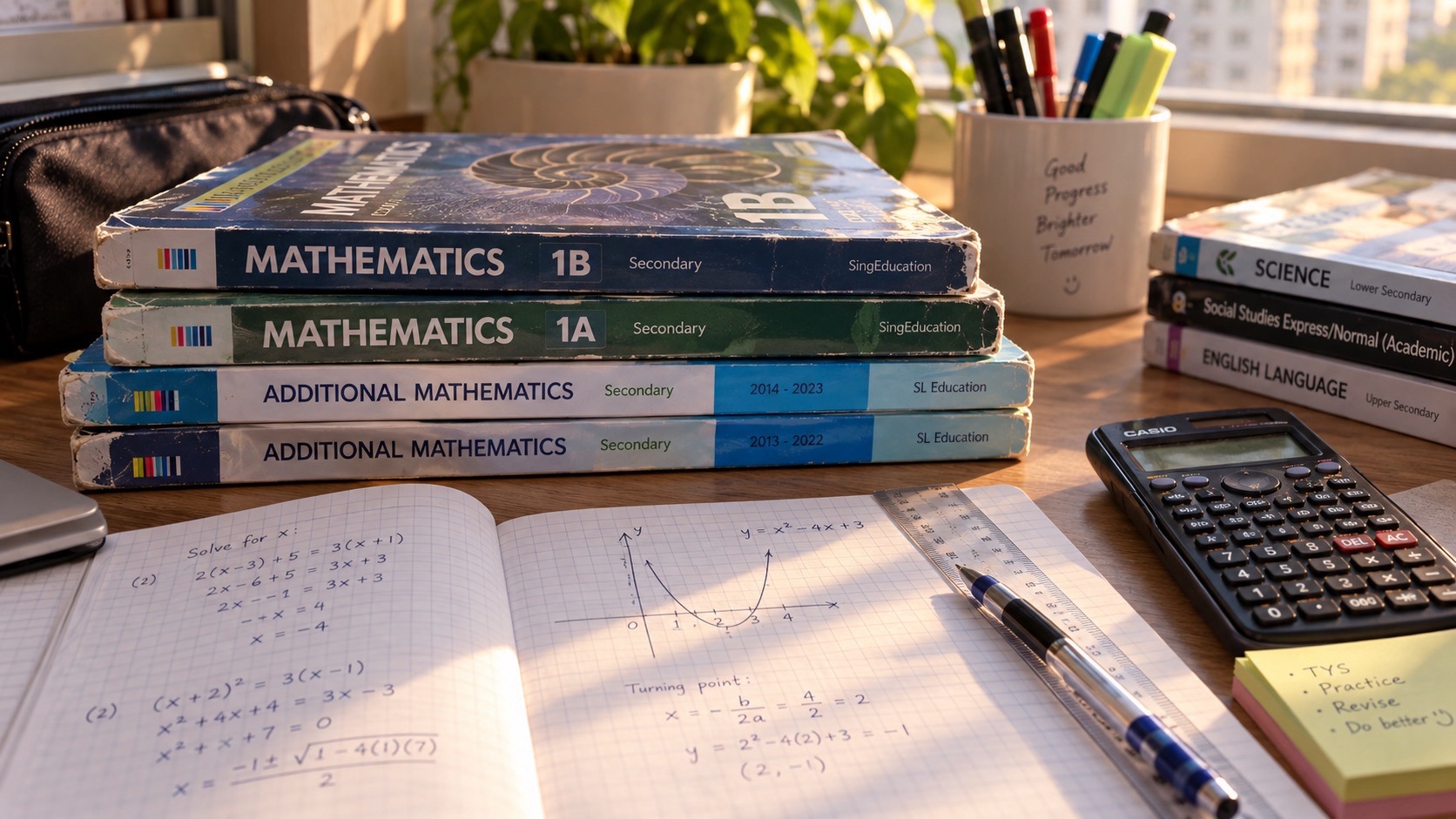
A Punggol student admitted through Posting Group 2 (PG2) can prepare for G2 Additional Mathematics by understanding differentiation as a way to describe a changing function’s gradient, then applying the power, product, quotient and chain rules to find tangent equations and identify stationary points. PG2 is an admission group; Additional Mathematics at G2 is a separate elective subject with its own SEAB syllabus, K232, and depends on the school’s actual offering and the student’s readiness. A derivative is not simply a symbol that makes powers smaller: it tells how a mathematical quantity changes, under appropriate conditions, and that meaning determines whether a calculated gradient is a maximum, minimum or neither.

SEAB’s 2027 G2 Additional Mathematics K232 syllabus contains differentiation of rational powers, products and quotients, the chain rule, gradient and normal calculations, connected rates of change, stationary points, second derivative classification and optimisation. Its two compulsory 1-hour-45-minute papers each carry 70 marks and 50% of the overall result. This article concentrates on the learner’s first incorrect derivative step and on worked tangent and stationary-point problems, rather than repeating the general Additional Mathematics course or area-under-curve guides already available in the eduKate ecosystem. The calculations below are original fictional examples; no real-world costs or measurements are asserted, and the graduating syllabus should not be mistaken for the immediate timetable of a child starting Secondary 1 in 2027.

• PG2 versus K232: entry group and individual G2 Additional Mathematics subject offer are distinct.
• Derivative: the instantaneous rate of change, or tangent gradient, where it exists.
• Power rule: d(xⁿ)/dx = nxⁿ⁻¹ for the relevant domain.
• Chain rule: differentiate the outer function and multiply by the inner derivative.
• Product rule: derivative of uv is u’v + uv’.
• Quotient rule: derivative of u/v is (vu’−uv’)/v² when v is nonzero.
• Tangent: use derivative gradient and a point to form a straight-line equation.
• Normal: a perpendicular line, with negative-reciprocal gradient where appropriate.
• Stationary point: a differentiable point where the first derivative is zero.
• Second derivative: can help classify maxima and minima, but a zero result needs further reasoning.
• Next step: differentiate a composite function and prove the gradient using a fresh tangent problem.

What PG2 means for Additional Mathematics

Posting Group 2 is an admission route into secondary school, not a lifetime ceiling or automatic elective assignment. Under Full Subject-Based Banding, eligible students may take particular subjects at different G levels. Additional Mathematics is a later offered subject, and the appropriate school subject-choice guidance determines availability. Families should not assume every student admitted through PG2 must take K232.

The examination year is another distinction. The 2027 K232 document is for candidates graduating in 2027. A child entering Secondary 1 in 2027 has a later graduation timetable and must build the current Mathematics prerequisites. Differentiation becomes useful after algebraic manipulation, powers and graph meaning are sufficiently secure. Appropriate sequencing is more productive than pushing a learner directly into final-year questions.

How this lesson differs from a generic calculus guide

The existing eduKate Additional Mathematics overview introduces differentiation, integration and the broad syllabus. This article owns a narrower practical challenge: correctly recognising a composite, product or quotient function and converting its derivative into a tangent or stationary-point interpretation. It is intended to help a teenager who already knows basic differentiation but makes systematic errors when expressions become layered.

A pupil may correctly derive x² but forget the inner derivative of (3x+2)⁴. Another may calculate a derivative yet confuse the tangent’s gradient with its y-intercept. Those weaknesses require targeted explanation, not a longer introduction to the word calculus.

The derivative describes how a function changes

For a smooth function y=f(x), the derivative f'(x) gives the instantaneous rate of change of y with respect to x, or the gradient of the tangent to its graph at a suitable point. A positive derivative indicates a locally increasing function, while a negative one indicates decreasing behaviour under the relevant interval conditions.

Ask what x and y represent. If y measures a fictional position and x is time, the derivative may represent velocity. If y is a geometrical function of length, the derivative has a different interpretation. The algebraic operation is the same, but the units and context change.

Average change is different from instantaneous change

The average rate of change between x=a and x=b is [f(b)−f(a)]/(b−a), where the denominator is nonzero. It is the gradient of a secant line between two graph points. The instantaneous derivative at a point concerns the limiting tangent gradient as the interval becomes small. The two values may differ for a curved function.

For y=x² between x=1 and x=3, average gradient is (9−1)/(3−1)=4. The derivative is 2x, so at x=1 the local gradient is 2 and at x=3 it is 6. The secant value lies between these in this case. This contrast makes the derivative’s meaning concrete.

A straight line has constant gradient

For y=3x+2, the derivative is three everywhere. The function is linear and its gradient does not change with x. For y=x², the derivative is 2x, so the gradient varies across the graph. The distinction explains why one constant rise-over-run can describe an entire straight line but not an entire parabola.

Ask the learner to identify the type of graph before differentiating. If a line’s derivative varies with x in a simple linear problem, something went wrong. This is an easy reasonableness check that protects later calculations.

The power rule is the first efficient method

For f(x)=xⁿ, the basic power rule gives f'(x)=nxⁿ⁻¹ over the relevant domain. Examples include x³ becoming 3x² and x⁵ becoming 5x⁴. The coefficient moves to multiply the expression while the exponent decreases by one. The rule is not the same as simply subtracting one from the final value of the function.

Ask the child to compute both y and dy/dx at a chosen input. For y=x³ and x=2, y=8 but dy/dx=12. The derivative is a gradient, not the new y-coordinate. This distinction prevents a common interpretation error.

Constants have zero derivatives

A constant function y=7 does not change as x varies, so its derivative is zero. For y=x²+7, the derivative is 2x because the added constant shifts the graph vertically without changing its tangent gradients. A pupil who carries +7 into the derivative as if it remained an x-term has misunderstood the meaning of a constant.

Ask whether the function’s output changes because of the constant alone. No change in x produces a change in that fixed contribution. Graphically, y=x² and y=x²+7 have corresponding tangents of equal gradient at the same x.

Constant multiples remain attached

If y=5x⁴, then dy/dx=5×4x³=20x³. The constant multiplier five remains and multiplies the derivative of x⁴. A student who writes 4x³ because they forgot the coefficient changes the scale of every gradient by a factor of five.

Ask the child to separate the multiplier from the variable part before differentiating. This pattern holds for sums and differences of eligible terms. A clear written step helps when a function contains several different powers and coefficients.

Negative and fractional powers need careful domains

The K232 syllabus includes differentiation of xⁿ for rational n, where the function and derivative are defined. For y=x⁻², dy/dx=−2x⁻³, or −2/x³ for x≠0. For y=√x=x¹ᐟ², the derivative is 1/(2√x) where x>0 for the ordinary real formula.

Ask the learner to distinguish the exponent rule from the domain restriction. Writing a formal expression is not enough if it is undefined at the input requested. Rational powers sometimes introduce roots and denominators, so domain awareness remains important.

Convert radicals to powers where useful

A square root can be written as a fractional power for differentiation. For y=√x, use x¹ᐟ² and apply the power rule to obtain (1/2)x⁻¹ᐟ². This is equivalent to 1/(2√x) for positive x. The conversion makes the familiar rule applicable to a new-looking expression.

Ask why the exponent one half becomes minus one half after subtracting one. An algebraic error here is often a fractions problem, not a calculus concept. The student should practise subtracting rational exponents accurately before handling nested radicals.

The chain rule handles functions inside functions

A composite function applies one function to the output of another. If y=[g(x)]ⁿ, the derivative is n[g(x)]ⁿ⁻¹g'(x) under suitable conditions. The extra factor g'(x) records how the inner expression changes. Omitting it is the most common mistake in first encounters with the chain rule.

Ask which part is inside. In y=(3x+2)⁴, the outer operation is raising something to the fourth power, while the inner expression is 3x+2. Differentiating the outer power alone gives an incomplete derivative. The inner gradient is three and must be included.

A complete chain-rule calculation

For y=(3x+2)⁴, let u=3x+2. Then dy/du=4u³ and du/dx=3. Multiplying gives dy/dx=12(3x+2)³. An incorrect answer 4(3x+2)³ has ignored the inner rate. Both expressions can look algebraically neat, so a check is important.

Ask the pupil to explain why three appears in the final coefficient. A chain rule is not simply an extra memorised line; it accounts for the fact that u changes three times as quickly as x under the linear inner expression.

A non-linear inner function needs its own derivative

Consider y=(x²+1)³. The outer derivative gives 3(x²+1)², while the inner derivative is 2x. Therefore dy/dx=6x(x²+1)². A student who multiplies by two rather than 2x has differentiated x² incorrectly within the inner function.

Ask the learner to write the inner and outer parts explicitly. The resulting expression does not need to be expanded unless the question requests it. Keeping it factored often makes stationary-point analysis or substitution simpler.

The chain rule works for negative powers

For y=(2x−1)⁻², differentiate the outer power to obtain −2(2x−1)⁻³ and multiply by the inner derivative two. The result is −4(2x−1)⁻³, with x≠1/2. Losing the negative sign or the domain restriction can make an otherwise valid method incorrect.

Ask what happens if x approaches the excluded value. The original function is undefined there, so one cannot assign a derivative at that point by substitution. Calculus still obeys the conditions of the underlying algebraic expression.

Nested functions require more than one chain step

An expression such as y=[(x²+1)³+2]⁴ contains more than one layer. Its derivative follows from differentiating the outer fourth power, then the inner cubic, then the x²+1 term. The result can be written 24x[(x²+1)³+2]³(x²+1)² under the relevant algebra.

Ask the pupil to trace the layers from outermost inward. A quick dimensional or numerical check can help catch a missing factor. The goal at G2 is understanding the chain of dependence, not expanding a complicated polynomial into dozens of unnecessary terms.

The product rule is not product of derivatives

For y=u(x)v(x), the derivative is u’v+uv’, not simply u’v’. This follows because both factors can change and each contributes to the product’s change. A student who writes derivative of x²(x+3) as 2x×1 misses two important terms.

Choose u=x² and v=x+3. Then u’=2x and v’=1, so y’=2x(x+3)+x²=3x²+6x. Expanding the original y=x³+3x² first gives the same derivative. Agreement between two methods is strong verification.

Product rule works with composite factors

Suppose y=x(2x+1)³. Let u=x and v=(2x+1)³. Then u’=1 and v’=6(2x+1)² by the chain rule. The product rule gives y’=(2x+1)³+6x(2x+1)², which can be factored as (2x+1)²(8x+1).

Ask which rule handles the outer multiplication and which handles the cubic inner expression. Students often know both separately but omit one when they appear together. A clear two-column setup for u and v can reduce this error.

Why factoring the derivative is sometimes helpful

A factorised derivative can make it easier to solve y’=0 when finding stationary points. In the preceding expression, y’=(2x+1)²(8x+1). Setting it equal to zero yields x=−1/2 or x=−1/8. The repeated squared factor has a different sign behaviour from the linear factor.

Ask whether the question needs a fully expanded polynomial or the values where the gradient vanishes. Factored form can be more informative for roots and sign analysis. Algebraic form should be selected according to the next mathematical task.

Quotient rule applies to a ratio of functions

For y=u(x)/v(x) with v≠0, the quotient rule gives y’=[vu’−uv’]/v². The order of terms in the numerator matters. A pupil who reverses the subtraction may obtain the negative of the correct derivative. A student who differentiates top and bottom separately and simply divides is generally incorrect.

Ask the learner to identify the numerator and denominator before using the formula. Put the subtraction in brackets to protect signs. A short check using an equivalent algebraic rewrite can reveal a mistake.

A worked quotient-rule example

Take y=(x+1)/(x−1), where x≠1. Set u=x+1, v=x−1, u’=1, v’=1. Then y’=[(x−1)−(x+1)]/(x−1)²=−2/(x−1)². The derivative is negative over its real domain, so the function is decreasing on each interval of continuity.

Ask why the numerator simplifies to negative two. Distributing the minus sign across the second bracket is essential. A student who obtains +2 has likely reversed the subtraction or missed a sign. This is a precise algebraic correction rather than a new calculus mystery.

Quotient rule and negative powers can agree

The same expression (x+1)/(x−1) can be rewritten as 1+2/(x−1) for x≠1. Differentiate the constant as zero and 2(x−1)⁻¹ using the chain rule to get −2(x−1)⁻². It matches the quotient-rule result.

Ask what the agreement tells the student. Two valid mathematical representations produce the same derivative over their common domain. This is a useful method check and strengthens the connection between algebraic manipulation and calculus.

Domain restrictions remain after differentiation

If the original function has a denominator zero at x=a, that point is excluded from the original domain. A derivative expression that appears algebraically simpler does not automatically restore the missing input. The same principle appears in algebraic fractions and equation solving.

Ask what the question provides and whether the requested point lies in the domain. A tangent cannot be assigned at a point where the function itself is undefined. Domain checks should precede substitution into any derivative formula.

A tangent touches the curve locally

The tangent line to a differentiable graph at a point has the same instantaneous gradient as the graph there. It can cross the graph elsewhere, so the everyday phrase touches only once is not a universal mathematical definition. Its important relationship is local agreement of gradient at the selected point.

Ask the pupil for the x-coordinate, the corresponding y-coordinate and the derivative’s value. All three are needed to write the line through that point. A gradient alone does not specify a unique tangent line without a point.

Find a tangent equation from a derivative

For y=x²+2x at x=1, the graph point is (1,3). The derivative is 2x+2, so the tangent gradient is four. The point-gradient equation y−3=4(x−1) simplifies to y=4x−1. The tangent is a straight line even though the original graph is a parabola.

Ask the child to verify the line passes through (1,3): substituting x=1 gives y=3. The gradient four comes from the derivative at x=1, not from the original function value. The two numerical results answer different questions.

The normal is perpendicular to the tangent

A normal line at a point is perpendicular to the tangent at that point. For nonzero finite tangent gradient m, the normal gradient is −1/m. In the preceding example, the tangent gradient is four, so the normal gradient is −1/4. The normal through (1,3) is y−3=−(1/4)(x−1).

Ask why changing the sign alone is insufficient. A gradient of −4 is not perpendicular to a gradient of four; their product is not −1. The correct relation is negative reciprocal. Horizontal and vertical cases require separate care.

Horizontal and vertical normal cases need care

If the tangent is horizontal with gradient zero, the normal is vertical and cannot be written as y=mx+c with a finite gradient. Conversely, a vertical tangent at a point may fall outside the ordinary differentiable model used in a simple question. A student who divides by zero while applying −1/m has ignored this special case.

Ask the pupil to sketch the local geometry. At the vertex of y=x², the tangent is horizontal y=0 and the normal is the vertical line x=0. The line equations are simple when the picture is understood.

A stationary point has first derivative zero

For a differentiable function, a stationary point occurs where f'(x)=0. The tangent is horizontal at that point. Stationary does not necessarily mean the graph has a maximum or minimum; an inflection can also have zero first derivative. The next step is to classify the point using suitable evidence.

Ask the pupil to separate finding the x-coordinate from evaluating the corresponding y-coordinate. If the task requests a coordinate pair, writing x=3 alone is incomplete. The function must be used to find y.

A quadratic minimum illustrates differentiation

Consider y=x²−6x+5. Its derivative is 2x−6. Setting y’=0 gives x=3, and substituting gives y=9−18+5=−4. The stationary point is (3,−4). Since the leading coefficient of x² is positive, the parabola opens upwards, suggesting a minimum.

The second derivative is y”=2, also confirming a local minimum under the ordinary second-derivative test. The result agrees with completing the square: y=(x−3)²−4. Different methods support the same geometric interpretation.

A negative quadratic has a maximum

For y=−x²+4x, the first derivative is −2x+4, zero at x=2. The point has y=−4+8=4. The second derivative is −2, indicating a local maximum. Completing the square gives y=−(x−2)²+4, which makes the same conclusion visible.

Ask the teenager to identify the sign of the second derivative and why it indicates curvature in the relevant local model. A stationary-point calculation becomes more meaningful when the answer is checked against the graph’s shape.

The second derivative describes gradient change

The first derivative measures a function’s rate of change, while the second derivative measures how that rate itself changes. In simple cases f”(x)>0 at a stationary point supports a local minimum and f”(x)<0 supports a local maximum. This test must be applied at a genuine stationary point in an appropriate differentiable setting.

Ask what physical interpretation is relevant. For a position function of time, second derivative can represent acceleration. For a generic curve it describes mathematical concavity. The symbol f” does not automatically mean an actual physical acceleration unless the function’s variables justify it.

A zero second derivative may be inconclusive

At a stationary point, f”(x)=0 does not automatically establish a maximum, minimum or inflection. For y=x⁴, the stationary point at x=0 is a minimum even though y”(0)=0. For y=x³, x=0 is a stationary inflection. Further sign analysis or a different method is needed.

Ask the pupil to compare values on either side of the point. The second-derivative test has a useful scope but not a universal decisive result. Understanding its limitation protects against an overly mechanical classification.

A stationary point of inflexion is possible

For y=x³, the derivative is 3x² and is zero at x=0. Yet the function increases on both sides of zero and does not have a local maximum or minimum there. The graph has a stationary point of inflexion. A child who automatically labels every zero derivative a minimum has missed this possibility.

Ask how the derivative’s sign behaves around x=0. It remains nonnegative on either side, unlike the sign change from negative to positive characteristic of a local minimum. Sign analysis complements the second derivative.

First-derivative signs can classify points

A function changing from decreasing to increasing as x passes a stationary point has a local minimum, while increasing to decreasing suggests a local maximum. If the derivative keeps the same sign, the stationary point may be an inflection under suitable conditions. The sign test is especially useful when f”=0 or complicated.

Make a sign table with intervals separated by stationary x-values. Ask the student to choose a valid test point on each interval. The resulting conclusions should follow the actual derivative signs, not a memorised shape assigned before calculation.

Optimisation needs a defined objective

Some K232 problems ask for a maximum area, minimum cost or another optimal value. Before differentiating, define the quantity to optimise as a function of one suitable variable and identify its domain. An algebraically valid stationary point can be irrelevant if it lies outside the permitted physical range.

Ask the learner what x represents. A length must usually be positive, and a number of objects may need to be a whole number. The best mathematical model is tied to the stated constraints. A beautiful derivative does not rescue a wrongly modelled objective.

A fictional maximum-height model

Imagine an invented mathematical model h(t)=12t−3t² for height in metres after t seconds within a stated physically suitable interval. The derivative h'(t)=12−6t is zero at t=2, where h(2)=24−12=12. The second derivative is −6, indicating a maximum of twelve metres under the model.

This is a classroom function, not a recommendation to launch or drop objects, and the numbers are not a measured Punggol event. Ask what the stationary time means and why a negative second derivative supports the maximum. The result should be interpreted within the assigned domain.

Tangent gradients can be negative

A negative derivative means the function is decreasing locally as x increases. If y=−2x²+1, then y’=−4x. At x=1, the tangent gradient is −4. A student who removes the negative sign because gradient must represent a positive speed has confused a generic mathematical slope with an unsigned physical quantity.

Ask how the graph behaves near x=1. It slopes downward to the right. Negative gradient is perfectly legitimate. Its practical meaning depends on what y and x represent, not on a rule that change must always be positive.

Derivative units help diagnose mistakes

If y is measured in metres and x in seconds, dy/dx is measured in metres per second. If y is square metres and x is metres, the derivative has units of metres. A result with incompatible units can indicate a wrong formula or a misinterpreted model.

Ask what division of quantities the derivative represents. For the fictional height function, h'(t) is a velocity-like rate, so its unit is m/s. The second derivative then has m/s². Dimensional reasoning makes calculus more understandable beyond symbol manipulation.

Connected rates use a new independent variable

Connected-rate questions may describe several quantities changing with time. For example, if area A of a square is x² and side length x changes over time, then dA/dt=(dA/dx)(dx/dt)=2x(dx/dt) under suitable conditions. The chain rule connects the changing quantities.

Ask which variable depends on which. If x is in metres and dx/dt in m/s, dA/dt has m²/s. A student who reports dx/dt as the area rate has skipped the dependence of area on side length. Correct notation makes the relationship visible.

A fictional changing-square example

Suppose a square’s side is six centimetres and increases at two centimetres per second at the specified instant. Area A=x², so dA/dt=2x(dx/dt)=2×6×2=24 cm²/s. This rate describes the instantaneous growth of area at that side length, not the new area after exactly one second.

Ask the learner to distinguish the current area, 36 cm², from its instantaneous rate of change, 24 cm²/s. They are different quantities. The exercise is abstract and does not assert physical growth of a real object.

A tangent is not an average over a large interval

On a curved graph, the gradient of the tangent at x=2 can differ from the average gradient between x=2 and x=5. A student who uses two widely separated curve points to find the tangent slope has generally calculated a secant instead. The derivative at the requested x gives the proper instantaneous gradient.

Ask whether the question says instantaneous, tangent or average. Words and symbols identify the intended relationship. This distinction links elementary straight-line gradients with the new calculus method without making them synonyms.

Graphical checks can expose a sign error

If a function’s graph is visibly increasing at the point, a negative tangent gradient may indicate the derivative has been calculated incorrectly or the graph read with reversed axes. A qualitative sketch can help check signs and stationary behaviour, although a rough sketch alone cannot prove an exact numerical gradient.

Ask the pupil to compare the derivative value with the expected local direction. Then check the algebraic steps. A graph is a diagnostic tool when interpreted carefully; it is not a substitute for valid differentiation.

A calculator does not replace the working

SEAB’s K232 assessment requires essential working to be shown, and provides relevant formulae and approved calculator use under specified rules. A student who enters an entire expression and copies a final numerical value without showing the chain or quotient rule may fail to demonstrate the required method.

Ask which intermediate expression supports the result. A good solution labels u and v where appropriate, writes the rule, differentiates, simplifies and interprets. The goal is transparent reasoning, not the longest possible algebraic expansion.

A fictional chain-rule misconception

Imagine a PG2-entry learner, Mira, differentiating y=(4x+1)³ and obtaining 3(4x+1)². Her tutor asks how quickly the inner 4x+1 changes with x. Mira adds the factor four and obtains 12(4x+1)². A new problem with a quadratic inner function then tests the same principle.

The story is fictional and does not guarantee an examination outcome. It demonstrates that a missing inner derivative is a specific conceptual error. Copying the corrected coefficient without understanding why it appears would not be a durable repair.

A fictional quotient-rule sign mistake

Imagine Daniel differentiating (x+1)/(x−1) and writing a positive two over the squared denominator. His tutor asks which term in the quotient numerator is subtracted. Daniel expands [(x−1)−(x+1)] to −2, correcting the sign.

On a changed fraction, Daniel should identify numerator, denominator and their derivatives before substituting. The correction targets distribution of a minus sign and the quotient structure, not a vague instruction to be more careful.

A fictional tangent-normal confusion

Imagine Farah finding tangent gradient 3 at a point and assigning normal gradient −3. Her tutor asks what relation perpendicular nonvertical lines satisfy. The correct normal gradient is −1/3. Farah then writes the normal through the known point with point-gradient form.

The example tests whether the learner understands a geometric relationship. A second point and different gradient check transfer. The student should also recognise special cases for horizontal and vertical lines rather than divide blindly by zero.

A fictional stationary-point classification error

Imagine Hana finding f'(2)=0 and immediately declaring a maximum without considering the derivative signs or curvature. Her tutor provides y=x² with a stationary point at zero, showing that zero derivative can correspond to a minimum. They then compare y=x³, which has a stationary inflection.

On a fresh function, Hana applies a proper test. The correction makes the classification evidence-based. A stationary point is a necessary starting condition for these smooth examples but not the whole argument.

Use an error log with meaningful categories

When marking Additional Mathematics work, record whether the error came from exponent arithmetic, chain-rule omission, product/quotient structure, sign distribution, domain restrictions, incorrect point coordinates or stationary classification. These categories guide the next short teaching exercise better than writing careless beside every wrong answer.

Ask the pupil to repair one category at a time and attempt a changed question a few days later. The aim is independent transfer. A correct final line copied from a model solution is not equivalent to understanding the derivative’s meaning.

A fourteen-day learning progression

Begin with gradients, powers and basic derivative rules. Next practise negative and rational powers, then simple composite functions with the chain rule. Move to product and quotient rules separately before combining them. In the second week solve tangent and normal equations, stationary points with second-derivative and sign tests, then simple optimisation and connected-rate problems.

This is optional preparation for a student actually offering the relevant Additional Mathematics course. It is not a compulsory Secondary 1 timetable. If factorisation or algebraic fractions are weak, repair them before demanding long calculus problems. Strong foundations reduce the number of simultaneous errors.

Where integration fits, and why this article stays focused

The K232 syllabus also includes integration as reverse differentiation and definite integrals for area under suitable curves. Those are important topics but not the central owner of this guide. The present learning goal is distinguishing derivative rules and using derivatives for tangents, stationary points and connected rates. A separate existing eduKate calculus guide already introduces integration and area.

Ask whether the child’s current task wants a rate or accumulated quantity. A derivative commonly describes rate of change, while an integral can describe accumulation under the relevant mathematical conditions. Choosing the operation follows the problem, not the fact that both belong to calculus.

The official paper format matters for readiness

For 2027 K232, both Paper 1 and Paper 2 last one hour forty-five minutes, each carries seventy marks and fifty per cent weighting. All questions are compulsory. The syllabus states three significant figures for non-exact numbers and one decimal place for degree angles unless instructed otherwise. Correct working remains important even when a calculator is used.

Parents should not copy the assessment structure of K210 G2 Mathematics or G3 Additional Mathematics without checking the relevant code. The current school and later examination cohort control actual assessment. An accurate preparation guide should separate subject choice, taught content and paper rules.

Official references and your next step

SEAB’s 2027 G2 Additional Mathematics K232 syllabus specifies derivatives of rational powers, product and quotient rules, chain rule, stationary points, tangent and normal gradients, connected rates, second derivative and optimisation. The official G2 directory confirms the K232 code and its separate elective status.

For algebraic fractions as a prerequisite, read the PG2 Algebraic Fractions guide. For the basic quadratic graph and stationary-point intuition, see the PG2 Quadratic Graphs guide. Your next step is to differentiate (3x+2)⁴, solve the tangent at x=1 for y=x²+2x, and classify the stationary point of y=x²−6x+5 using two different methods.

Frequently asked questions about PG2 G2 Additional Mathematics differentiation

Does PG2 entry guarantee G2 Additional Mathematics?

No. K232 is a later individual subject offer and school requirements apply.

What is the 2027 K232 paper format?

Two compulsory 1-hour-45-minute papers, each 70 marks and 50%.

What does the derivative mean?

The instantaneous rate of change or local tangent gradient where defined.

What is the derivative of x to the fifth power?

5x⁴.

Why does the chain rule include an extra factor?

It accounts for the rate of change of the inner function.

What is the derivative of (3x+2)⁴?

12(3x+2)³.

What is the product rule?

(uv)’=u’v+uv’.

How is a normal gradient found?

Use the negative reciprocal of a nonzero finite tangent gradient.

Is every stationary point a maximum or minimum?

No. Stationary inflection points also exist.

Does f”=0 prove there is no minimum?

No. The second derivative test may be inconclusive and another method is needed.

Editorial note, November 2026: All physical models and learners are fictional teaching examples. K232 is a later elective and the 2027 syllabus applies to that graduating cohort. Follow the current school lesson and check domain restrictions and units for every calculation.