
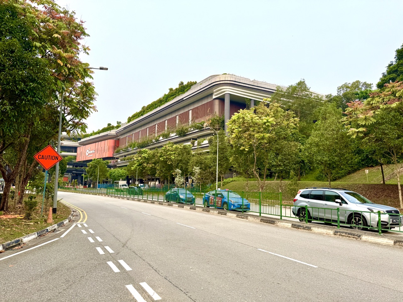
A badminton score, table-tennis rally count or observed waiting time can become a Statistics lesson when the learner records what was measured, who was included, when the data were collected and what a summary can legitimately tell us. ActiveSG Punggol Sport Centre at 11 Sentul Crescent began selected operations on 27 October 2026, ahead of its announced 22 November formal opening. The new gym and selected courts offer a recognisable sports context, but families do not need to purchase a booking or collect information about strangers to learn statistical thinking. A fictional five-game dataset, clearly identified as invented, is enough to show how a mean can hide variation, how a graph can mislead, and why a small convenient sample cannot speak for an entire neighbourhood.
The 2027 SEC G3 Mathematics syllabus K310 includes tables, charts, histograms, cumulative frequency diagrams, box plots, mean, median, mode, range, interquartile range and standard deviation, along with explaining how diagrams can mislead. Singapore’s official statistics-learning resources explain that even a sample with some matching demographic characteristics may omit important groups and produce bias. This article builds those ideas from sport. It is distinct from basic Primary Mathematics lessons on counting and fractions: here the focus is on study design, sampling, uncertainty, representation, fair comparison and the limits of inference. The numbers below are educational illustrations, not actual Punggol court usage, official ballot probabilities or private participant data.
- Place: Punggol Sport Centre, 11 Sentul Crescent; real availability only via MyActiveSG+.
- Statistical question: start by defining what the data are supposed to describe, such as rally length or a fictional group’s preferred session time.
- Units: participants, court-hours, rallies, attempts and minutes are different units and must not be mixed.
- Sample and population: five friends are a sample of five friends, not a representative survey of every Punggol household.
- Descriptive statistics: mean, median, mode, range, quartiles and spread summarise observed data in different ways.
- Displays: bar charts, histograms, dot plots, line graphs and box plots answer different kinds of questions.
- Caution: chart axes, selected time periods, uneven categories and hidden denominators can mislead.
- Inference: a relationship observed in data is not automatically proof of cause.
- Ethics: work with fictional numbers or voluntary private family observations; never scrape the booking portal or record strangers without permission.
- This guide: accurate worked examples, critique exercises, fair comparisons, data privacy and a four-week Statistics project.
Definition lock: statistics is reasoning from data
Statistics concerns collecting, organising, analysing and interpreting data to understand patterns while recognising uncertainty. Calculation is only one part. Before finding an average, ask what each number represents and how it was obtained. A five-point list from one child is not a population measure of national sporting performance.
A sensible statistical conclusion matches the study design. If a family records a few rally lengths during one practice, it can describe those specific rallies. It cannot automatically establish a typical result for all badminton players, every court, or future sessions.
The important habit is to move from a clear question to appropriate data and then to a cautious interpretation. Statistics is not just the ability to press an average button on a calculator.
Why this is different from a Primary sports-Maths article
Counting points, simplifying fractions and reading a simple bar chart are valuable Primary-level tasks. This article goes further by asking whether the data collection was fair, whether comparisons use compatible groups, whether the selected statistic hides important differences, and how confidently a conclusion applies beyond the observations.

For example, two groups might both average six rally returns, but one group could perform consistently near six while another alternates very short and very long rallies. Their means match, yet their experiences differ. We need a measure of spread and the original data to see that difference.
The aim is deeper analytical understanding, not simply more difficult arithmetic. A correct calculation can still produce a misleading argument when the sample or interpretation is weak.
Start with an answerable statistical question
“Is sport good?” is too broad for a short investigation. “What were the rally lengths in ten cooperative attempts by our family on Saturday?” is clearer. It defines the activity, the measurement and the observations. “Which booked courts are most popular in all of Singapore?” would require much more comprehensive and properly sourced data.
Choose a question suited to the available information. A student might investigate the spread of fictional rally lengths or compare two invented practice sessions. If gathering real family observations, obtain agreement and keep the data private.
A good question determines which information matters. Without it, students may collect an impressive spreadsheet that cannot answer anything useful.
Define the unit of observation
A dataset needs an observational unit: the thing being counted or measured. One row might represent a rally, one booking attempt, one player or one court-hour. These are not interchangeable.
Suppose a student writes ten rows of rally lengths. Those represent ten rallies, not ten different players. Saying “ten players averaged six returns” would be false. Likewise, the number of court bookings is not the same as the number of unique individuals who used them.
Label each table carefully. A simple heading such as “Rally number” and “Number of returns” prevents a surprising amount of confusion later.
Define the target population
A population is the full group about which the investigator wants to make a claim. If a study asks about all Punggol households, its population is very different from a study asking about one family or the participants in a single sports club.
An investigation becomes unreliable when the population is expanded after the data have been collected. A survey of six classmates cannot automatically be described as a survey of “Punggol residents” without serious limitations.
The official Singapore statistics guidance explains why representative sampling requires care. The first step is to define whom the study is about, rather than finding available respondents and retroactively claiming they represent everyone.
Sample size matters, but size alone is not enough
A sample of fifty people may provide more information than a sample of five, but it can still be biased if all fifty belong to the same sporting club and the researcher wants to describe all residents. Conversely, an appropriately selected smaller sample may be informative for a narrower question.
The way a sample is chosen matters alongside its size. People who volunteer for a sports questionnaire may be more interested in sport than those who decline. Interviewing only visitors present at 7pm may omit residents who work evenings.
Statistics requires thinking about which groups could be missing, not merely displaying a large number of responses.
Convenient samples can miss important groups
Imagine a student asking the first twenty people seen near a badminton court which sport they prefer. Such a sample will probably contain people already interested in that part of the venue. It may under-represent swimmers, people who do not book courts, residents with mobility barriers and families who cannot attend at that hour.
The Ministry of Manpower’s statistics-learning pages warn that selecting people from one convenient location can leave out important groups even when certain visible demographic proportions match.
A school project should not approach strangers without appropriate permission anyway. Use a fictional survey to explore the issue and explain why a convenience sample has limited reach.
Self-selection can distort an online poll
A social-media poll attracts people who see it and decide to respond. Residents who are not on the platform, dislike the topic or ignore the post will be absent. This can produce a pattern reflecting audience interest as much as underlying population preference.
A poll asking “Do you love the new sports centre?” may also influence responses by its wording. Neutral questions help, but voluntary online participation still has selection limitations.
Do not treat a hundred enthusiastic replies as proof that every Punggol resident agrees. A percentage requires a known population or clearly described sample and a defensible method.
Bias is not the same as deliberate dishonesty
Statistical bias can arise from the sampling method, question wording, measurement process or missing responses. It does not always mean the researcher intended to deceive. An honest student may mistakenly sample only friends, because they are easy to reach.
The correct response is to identify the limitation and improve the method where appropriate. If the sample cannot support a town-wide conclusion, reduce the scope of the claim rather than accuse everyone involved of bad faith.
This distinction helps students learn from design errors. Statistics becomes stronger when limitations can be acknowledged without embarrassment.
Define a rally consistently
Suppose one student counts the serve as the first hit, while another counts only returns after the serve. Their “rally length” measurements will differ even if they watch the same sequence. Agree on the definition before collecting data.
A class might define rally length as the total number of legal racket contacts from a valid serve through the point’s end. Another definition could be valid for a particular study if explained clearly. The crucial requirement is consistency.
Do not quietly change the definition after seeing the results. A consistent measurement protocol matters more than a table full of apparently precise numbers.
Missing data should not become zeros automatically
If a rally length was not observed because the recorder looked away, that is missing information, not a confirmed zero-length rally. Replacing unknown values with zero can pull the average downward and create an inaccurate picture.
A small dataset can mark the observation as “missing” and explain the reason. The student may decide to report the number of usable observations separately. They should not silently invent values to complete the spreadsheet.
This principle transfers to school assessment data, surveys and business records. A blank measurement does not automatically mean the phenomenon was absent.
Use one fictional dataset consistently
Consider five invented rally lengths: 4, 6, 5, 9 and 6 returns. These are not results from actual Punggol players. The total is 30 returns, and there are five rallies. The mean is therefore 30 ÷ 5 = 6 returns per rally.
Write down both the number and its unit. The average describes the five observations under the chosen definition, not the expected result for every future game.
A statistic becomes useful only when a reader can trace where it came from. A correct total, count and unit provide that trace.
Mean versus median
For 4, 6, 5, 9, 6, order the numbers as 4, 5, 6, 6, 9. The middle value is 6, so the median is six. The mean was also six. In this example, the two measures agree, but they are not calculated in the same way and do not always match.
The mean uses all numerical values and can be influenced by an extreme observation. The median identifies the middle of an ordered dataset. Each can be more useful in different contexts.
Students should explain what the measure describes rather than memorise that one is universally better. The right choice depends on the question and distribution.
Mode tells a different story
In the same dataset, six appears twice while the other numbers appear once. Therefore the mode is 6. Mode describes the most frequently occurring value, not necessarily the middle or average. A dataset can have more than one mode or no single unique most-common value.
In a larger set of rounded rally lengths, a mode can describe a common outcome. But grouping and rounding may change the result, so the measurement rules should remain visible.
Mean, median and mode answer related but distinct questions. Using all three does not automatically make the study more scientific if none addresses the research question.
Range is a first measure of spread
The smallest observed rally length is four and the largest is nine. The range is 9 − 4 = 5 returns. Range provides a simple view of spread using only the extremes.
However, the range ignores all the other values. A dataset of four, six, six, six and nine has the same range as four, five, six, six and nine but a different distribution. Both facts matter.
Students should learn that no one summary captures an entire dataset. A good chart or table often remains helpful alongside the chosen statistic.
Compare groups with identical means
Consider two invented groups. Group A has rally lengths 6, 6, 6, 6, 6, while Group B has 2, 4, 6, 8, 10. Both total thirty across five rallies and both have a mean of six. Yet Group A shows no variation while Group B has a range of eight.
A claim that the groups performed “the same” because their means match hides the obvious difference in consistency. The appropriate conclusion depends on whether the question concerns average length, predictable repetition or variation.
This example shows why statistical spread is meaningful and why readers should ask for the original data when a headline offers only an average.
Quartiles divide ordered data
Quartiles help describe the distribution by identifying values around the lower and upper parts of an ordered dataset. The exact calculation convention can depend on syllabus and dataset method, so students should follow the specified school approach and state it where needed.
For an odd-sized ordered list, different teaching conventions may exclude or include the median when finding lower and upper halves. This can affect reported quartiles in small samples. Do not hide the method when precision matters.
The purpose is to understand how the middle fifty per cent of a distribution can be described, not simply to produce two unexplained numbers.
Interquartile range is not the full range
The interquartile range, or IQR, is upper quartile minus lower quartile. It describes the spread of the central portion of the ordered data rather than the distance between the minimum and maximum.
It can be helpful when extreme values distort the overall range. But it too omits information, particularly about the tails. A student should not claim that IQR alone reveals every interesting feature of a dataset.
The 2027 G3 Mathematics syllabus explicitly includes quartiles and interquartile range. Students should practise both calculation under the required convention and interpretation in plain language.
Standard deviation summarises variation
Standard deviation is a measure of how dispersed numerical values are around their mean, calculated using a specified formula. A dataset with identical values has zero standard deviation under the usual definitions. A more variable dataset generally has a larger value, though comparisons require compatible units and contexts.
Older Secondary students may calculate standard deviation for grouped or ungrouped data according to the actual syllabus. Beginners should first understand the concept through contrasting datasets rather than memorising a calculator procedure without meaning.
A small standard deviation is not automatically proof of better sporting skill; it simply describes spread under the chosen measure.
A dot plot shows individual observations
A dot plot places marks at the measured values, allowing readers to see clusters, gaps and repeated outcomes. For the fictional rallies 4, 5, 6, 6 and 9, place one dot over four, one over five, two over six and one over nine.
The plot immediately shows why six is the mode and where the longest observation lies. It can also make outliers easier to notice in a small dataset.
Always label the axis and unit. Without the title “Returns per rally,” the dots could be mistaken for minutes, points or player ages.
A bar chart is useful for categories
A bar chart compares frequencies or values across distinct categories, such as the number of participants choosing badminton, pickleball and table tennis in a fictional class poll. Categories should be defined and counted consistently.
It is usually misleading to present categories with unequal bar widths as though width has no meaning. A proper bar chart also needs readable labels and a suitable numerical scale.
Do not treat a bar chart of a small class as evidence of island-wide preferences. The graph displays the collected values; it does not repair a weak sampling method.
Histograms display grouped numerical data
A histogram is used for a numerical distribution divided into intervals. Bars ordinarily touch because the intervals represent adjacent ranges on a scale, unlike a bar chart of separate sport categories.
If the class intervals have equal widths, the heights can correspond to frequencies under the standard basic approach. If interval widths vary, frequency density becomes important to represent frequencies fairly through area. Students should follow the method relevant to their level.
A chart that looks superficially similar to a bar chart may convey a different structure. Interpreting the variable type is as important as reading the numbers.
Interval boundaries must not overlap
Suppose rally durations are grouped into 0–4 seconds, 5–9 seconds and 10–14 seconds, for observations recorded in whole seconds. Those bins are clear for integer values. But writing 0–5 and 5–10 without explaining boundary inclusion makes the value five ambiguous.
For continuous measurements, define intervals using appropriate non-overlapping boundaries such as [0,5) and [5,10), and explain what the notation means. A student should not rely on a label that leaves observations unassignable.
Small category choices can change a distribution. Clear definitions make the analysis reproducible.

A line graph needs an appropriate time axis
A line graph can show repeated measurements over ordered time points, such as a fictional group’s average rally length across four weeks. The horizontal axis should identify the dates or weeks, while the vertical axis describes the measured quantity.
Connecting points with a line can suggest a progression between observations, but it does not mean that every unmeasured moment followed the line exactly. A graph can also appear more dramatic when vertical bounds are truncated.
Ask students to inspect units, spacing and whether the line represents observed data or an inferred trend. A chart is a communication choice, not a substitute for statistical judgement.
Truncated axes change visual impressions
Imagine two bars representing averages of 98 and 100. If the vertical axis starts at zero, the difference appears small relative to the values. If it starts at 97, the visual gap can look enormous. The underlying two-point difference is unchanged.
Truncated axes are not automatically illegitimate in every chart type, but they need clear labels and appropriate justification. A bar chart that uses area or height to suggest magnitude can become especially misleading when the baseline is hidden.
The 2027 SEC Mathematics syllabus explicitly expects students to explain why a diagram may lead to misinterpretation. This is a practical example of that skill.
A pie chart must represent a whole
A pie chart divides a complete total into categories that collectively account for the whole under a specified definition. If a survey allows every person to choose multiple sports, the sum of category selections may exceed the number of respondents. A simple pie chart of those overlapping choices would be misleading unless the data are handled appropriately.
Ask whether categories are mutually exclusive and what the denominator represents. If a person can choose both badminton and table tennis, the counts are not naturally a single-partition breakdown of people.
A chart should match the structure of the question, not be chosen simply because it looks attractive.
Box plots compare distributions compactly
A box-and-whisker plot summarises a distribution through positions such as median, quartiles and whiskers under a defined convention. It can help compare groups without displaying every observation individually.
However, different box plot conventions can handle whiskers and outliers differently. Students should understand the school-taught convention and avoid inferring an exact mean when the chart does not show it.
A box plot is especially useful for comparing spread and central position, but sample sizes and context still matter. Two boxes that look similar do not automatically imply identical underlying populations.
A percentage change needs a baseline
Suppose a fictional activity group records ten successful attempts in week one and twelve in week two. The absolute change is two attempts. Relative to week one’s ten, the percentage increase is (12 − 10) ÷ 10 × 100 = 20%.
That does not mean the success rate improved by twenty percentage points. We would need the number of attempts in each week to calculate success rates. If week two involved far more attempts, the interpretation may change.
Students should distinguish absolute change, relative change and percentage-point change. The words sound similar, but they answer different questions.
Success totals are not success rates
Imagine Player A succeeds on 8 of 10 attempts and Player B succeeds on 12 of 20. Player B has more total successes, but the success proportions are 80% for A and 60% for B. Neither number alone establishes who is better overall; difficulty and conditions may differ.
A fair comparison states what is being compared. If the objective is total completed tasks, the count matters. If the objective is proportion of attempts, the denominator is essential.
Avoid posting a child’s personal success rate as a public ranking. Use anonymous or fictional data to learn the mathematics.
Repeated observations are not independent people
If one student plays twenty rallies, those are twenty rally observations from a single person, not twenty separate participants. Treating them as twenty independent people can exaggerate the evidence about individual variation.
The distinction matters when generalising. A strong player completing many rallies may dominate a dataset of results, leaving little information about other learners.
Ask what the observational unit is and how observations cluster within players, sessions or conditions. This is a valuable preparation for more advanced statistical reasoning.
Correlation is not causation
A group might notice that longer practice sessions and longer rallies occur together. This does not automatically prove that extra practice duration caused the improvements. More experienced players may choose longer sessions, equipment may differ, and many other factors can influence the data.
A relationship is a finding that two variables move together under observed conditions. A causal claim needs more careful design and evidence.
Students should avoid writing “proves” whenever a graph shows two lines increasing. The honest wording is often “is associated with,” followed by plausible explanations and limitations.
Why an opening-week sample may mislead
The new Punggol centre may attract curious first-time visitors in its opening weeks. A survey conducted only in that period could over-represent people excited by new facilities and under-represent those who have not yet visited.
It would be misleading to use that sample to predict attendance in every month of 2027 without appropriate longitudinal evidence. The location, season, school holidays, programme status and promotional conditions may change.
A good report dates the sample and explains why the period may be unusual. Context is part of data quality.
Beware comparing non-identical time windows
A crowd count from Friday 7pm should not be directly equated with a Tuesday 10am count as proof of one venue’s permanent popularity. The day, time, season and operating status differ.
If the goal is to compare two venues, collect observations across comparable periods using the same definitions. Even then, weather, school events and closures may influence results.
The correct lesson is to design comparable observations before judging which group or facility has more demand. More numbers do not fix an inconsistent comparison.
How to discuss outliers
An outlier is a value notably different from the others under the chosen context and method. A very long rally could be a genuine exceptional observation, a recording mistake or a result of unusual conditions.
Do not automatically delete it because it makes the chart look inconvenient. Check the record, understand the cause where possible and explain any exclusion rule. Sometimes reporting results both with and without the extreme observation is informative.
The purpose is transparent reasoning rather than forcing data to support a preferred conclusion.
Why quartiles and mean should be used together carefully
Quartiles describe positions in ordered data while the mean summarises numerical magnitude. Both can help compare distributions, but they have different sensitivities to extreme values. A group with a few unusually long rallies might have a higher mean without a similarly large change in median.
Students can draw two invented distributions, compute appropriate summaries and describe what each reveals. They should avoid deciding that whichever statistic makes their preferred group look stronger must be the “correct” one.
A good analyst chooses the measure in response to the question and explains its limitations, not in response to the answer they want.
Official data and fictional data have different uses
A public SportSG facility page may provide confirmed prices or booking rules. An invented rally dataset helps teach a statistical technique. The two should never be presented as the same kind of evidence.
If a student calculates a 20% improvement from fictional numbers, label the calculation hypothetical. If they quote published court rates, include the date and eligibility category.
Clear source separation allows rich examples without falsely implying that the operator has released personal performance or facility-usage data.
Do not scrape the booking portal for school research
MyActiveSG+ is a real booking and account service, not an unrestricted dataset for student scripts. Do not build automated requests, bots or unofficial tools to collect availability in bulk or access other users’ data. SportSG’s no-onselling and anti-bot policies protect shared public facilities.
Use invented records offline or officially published aggregated statistics where appropriate. A meaningful Statistics project does not depend on harvesting private information.
Technical curiosity must operate within legal, ethical and operator restrictions. A clear fictional dataset is often a better learning resource because the assumptions are fully controlled.
Statistical privacy for children
A child may feel uncomfortable having every miss, score or movement measurement recorded. Respect that preference. A family can use anonymous invented numbers or count a cooperative task without linking the result to a person’s identity.
Never publicly post images of other children, booking QR codes or personal health data as part of a school chart. If real voluntary data are collected, explain the purpose and who will see it, and keep the scope minimal.
Good statistics includes responsible collection and use. A precisely computed average is not valuable if the process harms the people being studied.
A hypothetical class survey
A fictional class of twenty pupils is asked to choose exactly one preferred racket sport. Eight choose badminton, five pickleball, four table tennis and three tennis. The totals add to twenty. A bar chart and a pie chart could describe this fictional class under that defined single-choice question.
It would be wrong to say “40% of Singapore prefers badminton” because eight out of twenty pertains only to the invented class. Also, if the question allowed multiple responses, the chart design and denominator would need reconsideration.
This exercise teaches students to connect a number with the group it actually describes.
A second hypothetical class with different results
Suppose another fictional class of twenty pupils chooses four badminton, eight pickleball, five tennis and three table tennis. Combined across both classes, badminton receives twelve of forty responses, or 30%. But the preferences differ between the classes.
An overall percentage may hide variation across groups. A student should consider showing both class distributions before using the combined result.
This is not a claim about actual schoolchildren in Punggol. The example demonstrates that aggregation is a decision which may conceal important distinctions in the data.
A misleading chart challenge
Draw a fictional bar chart of two session satisfaction averages, 4.0 and 4.2 on a five-point scale. Make one version with a vertical baseline at zero and another beginning at 3.9. Ask what impression each creates and which axis choice is appropriately labelled for the intended purpose.
The numerical difference is 0.2 points regardless of the visual presentation. A dramatic-looking chart does not increase the measured difference.
The exercise should remain fictional, not a public rating of actual SportSG staff or programme participants. Its aim is to teach visual honesty.
A sports case study with mixed groups
Two groups practise badminton for different durations. One consists mainly of beginners, while the other includes experienced players. Their mean rally lengths differ. Without accounting for playing level, equipment and practice conditions, we cannot attribute the difference to the time of day or hall quality.
The student should list the possible confounders and propose what information a more careful study would require. A stronger comparison may involve the same group under similar conditions, though even then other changes can occur.
This scenario demonstrates how statistical design influences interpretation. The most interesting conclusion can sometimes be that current evidence is insufficient.
A four-week Statistics investigation plan
Week one: define one fictional sports question, its population, variables and observational units. Week two: collect or construct a small clearly labelled dataset and calculate mean, median and spread. Week three: create two appropriate displays and one deliberately misleading variant with a clear educational label, then critique the difference. Week four: write an interpretation naming possible bias, uncertainty and the limits of inference.
Do not conduct invasive surveys or scrape live bookings. Use school-appropriate tools and datasets under supervision where needed. The purpose is to learn good methods, not manufacture impressive numbers.
A completed project should explain its assumptions, sources and limitations at least as clearly as its calculated answers.
Common mistakes in sports Statistics
Do not treat one player with twenty rallies as twenty distinct participants. Do not compare rates without denominators. Do not assume the same mean implies the same consistency. Do not create histograms with overlapping categories. Do not hide truncated axes. Do not claim an observed association proves causation. Do not infer all Punggol residents’ preferences from a small self-selected sports group.
Another mistake is using the most complicated statistic available simply to appear advanced. Choose the measure that addresses the real question and explain why it is appropriate.
Clear, honest analysis is more useful than a graph crowded with decorations and unsupported conclusions.
Frequently asked questions
Is this the same as learning Primary Mathematics through sport? No. This guide focuses on sampling, bias, statistical spread, visual interpretation and inference, building on basic data skills.
Does a mean describe every observed rally? No. It summarises the dataset and can hide substantial variation.
What is the difference between sample and population? The sample contains collected observations; the population is the complete target group of interest.
Can twenty volunteers represent all Punggol residents? Not automatically. Selection methods and missing groups affect representativeness.
Why are truncated graph axes risky? They can exaggerate visual differences when the scale or baseline is unclear.
Does correlation prove a training method worked? No. Other factors or selection effects may explain an association.
Is a box plot the same as a mean graph? No. Box plots summarise order positions and spread; the mean may not be shown.
Can we calculate true ActiveSG ballot winning odds from a fictional example? No. The real probability requires appropriate actual application and allocation information.
Is it acceptable to use invented data? Yes, when clearly labelled as hypothetical educational data and not presented as real findings.
May students scrape court availability to build a dataset? Do not do so. Use authorised published information or offline invented records.
Official sources and your next step
Read the SEAB 2027 G3 Mathematics syllabus K310 for the actual statistics and probability topics. The MOM statistics learning guide explains sampling limitations; the Singapore Department of Statistics data basics distinguishes survey and administrative data. Use MyActiveSG+ for real sports access, not for unofficial bulk collection. For distinct younger-level maths learning, see our Primary Mathematics sports examples.
Your Next Step: take a small fictional dataset and state the question, unit, group, mean and measure of spread. Draw one honest display and explain one way it could mislead if the axis or sample were changed. The quality of Statistics lies in what the evidence supports, not just in the calculation.
Editorial note: Prepared 1 November 2026. All sample counts and survey results are fictional. No claims are made about actual Punggol court usage, children’s performance, real ballot probabilities or private operator statistics.


